How to Use AGGREGATE Function in Excel?
Overview
The aggregate of a data table or list is returned by Excel's AGGREGATE function. A function number serves as the first argument, while various data sets make up the other arguments. One needs to remember the function number to know which function to use.
AGGREGATE function is classified as a Math/Trig Function. In Excel, it can be utilized as a worksheet function (WS). The AGGREGATE function can be used as part of a formula in a worksheet cell as a worksheet function. Microsoft developed it to solve the drawbacks of conditional formatting. In several cases, conditional formatting cannot be used if the range contains errors. You can ignore mistakes or concealed rows when using the Excel AGGREGATE function.
What is Data Aggregation in Excel?
The AGGREGATE function is intended for vertical ranges or columns of data. It is not intended for horizontal ranges or rows of data. For instance, hiding a column has no impact on the aggregate sum value when subtotaling a horizontal range with option 1, such as AGGREGATE(1, 1, ref1).
AGGREGATE Function in Excel
The output of an aggregate calculation, such as AVERAGE, COUNT, MAX, MIN, etc., made on one or more references, is returned by the AGGREGATE function. The AGGREGATE function offers more computation possibilities and more flexibility over disregarding particular things. It is similar to an updated version of the earlier SUBTOTAL function. Compared to other functions that carry out identical activities, the AGGREGATE function is particularly helpful for two reasons:
There are several choices in AGGREGATE for ignoring errors, concealed rows, and other possible functions in data.
Aggregate function Excel can natively handle a variety of array operations. There are 19 functions that AGGREGATE can execute in total, and the function to be executed is specified as a number that appears as the function's first argument, function num. Options, the second input, determines how AGGREGATE handles mistakes and values from concealed rows. Function num, options, ref1, and ref2 are the four arguments required by the AGGREGATE function. Only the first three arguments—function num indicates the operation, options settings various behaviours, and ref1 is the array of values to be processed—are necessary for the first 13 supported functions.
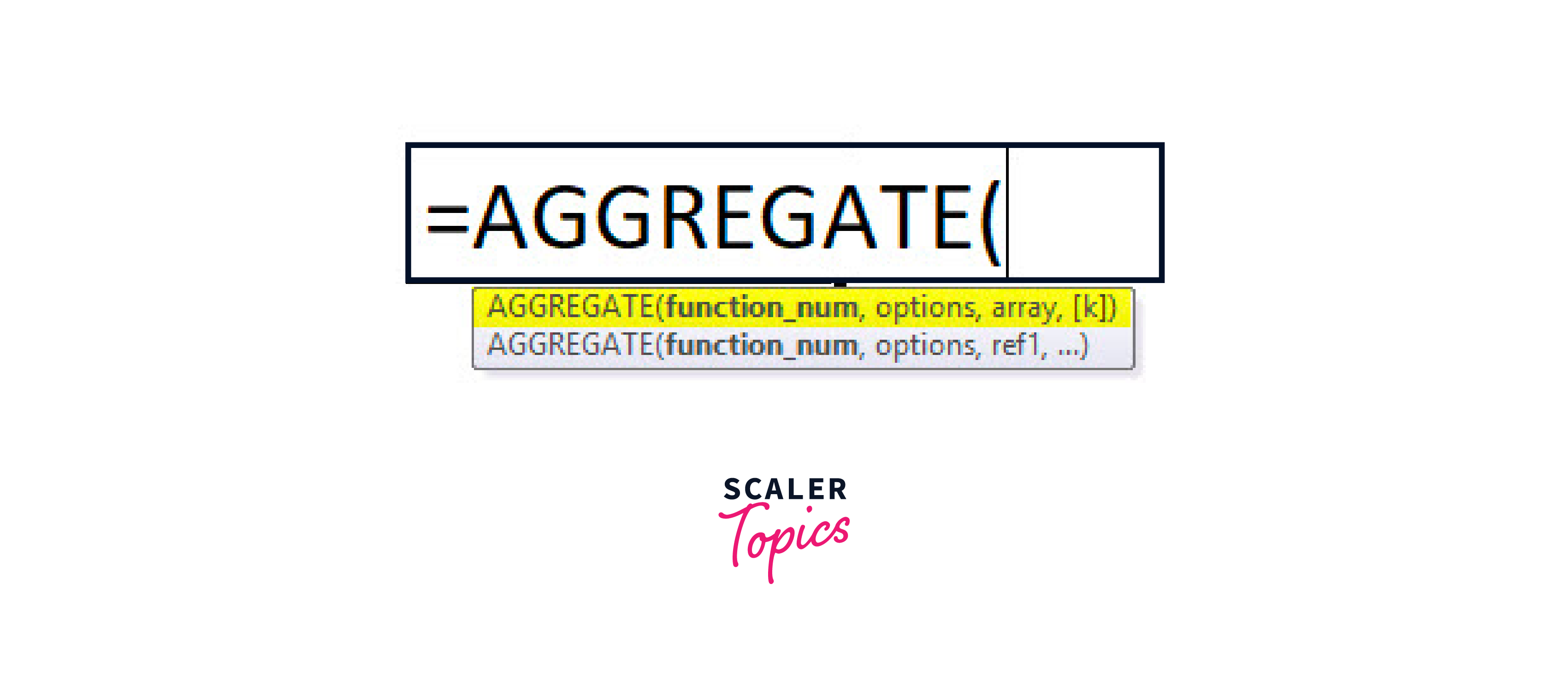
Syntax
The aggregate function Excel has two syntaxes:
-
Array Syntax
The Microsoft Excel AGGREGATE function's ARRAY syntax is as follows: AGGREGATE( function, options, array, [optional_argument] )
-
Reference Syntax
The Microsoft Excel AGGREGATE function's REFERENCE syntax is as follows: AGGREGATE( function, options, reference1, [reference2], ... )

-
Arguments
a. function: Any of the following values can represent the function you want to use:
Value Function 1 AVERAGE 2 COUNT 3 COUNTA 4 MAX 5 MIN 6 PRODUCT 7 STDEV.S 8 STDEV.P 9 SUM 10 VAR.S 11 VAR.P 12 MEDIAN 13 MODE.SNGL 14 LARGE 15 SMALL 16 PERCENTILE.INC 17 QUARTILE.INC 18 PERCENTILE.EXE 19 QUARTILE.EXE b. reference:1 When utilizing the REFERENCE syntax, reference1 is the function's first numerical parameter.
c. reference2: When using the REFERENCE syntax, the function will accept the numeric arguments 2 through 253.
d. array: When using the ARRAY syntax, an array, array formula, or a reference to a set of cells.
e. optional argument: When utilizing the ARRAY syntax, a second argument is necessary when using the LARGE, SMALL, PERCENTILE.INC, QUARTILE.INC, PERCENTILE.EXC, or QUARTILE.EXC.
Return Value
The result of the aggregate function excel is a number.
Examples
Return the MAX Value in the Range
To return the MAX value in the range A1
Return the MIN Value
To return the MIN value with the same options, change the function number to 5: =AGGREGATE(5,7,A1:A10) // min value
Nth Largest
The formulas in D8
Here, the LARGE function is run by the function number 14, which is present. The k argument, which is necessary for the BIG function, is listed as the final argument in the three formulations above.
Array Operation
The fact that AGGREGATE can handle arrays directly when the function number is 14–19 makes it especially helpful for more complicated formulas. For instance, you could use AGGREGATE as follows to get the MAX value on Mondays with data that includes dates and values: =AGGREGATE(14,6,values/(TEXT(dates,"ddd")="Mon"),1) Here, we specify 6 for the option and 14 for the function (HUGE) (ignore errors). The TEXT function is then used to create a logical expression that will check all dates for Mondays. An array of TRUE/FALSE values that serve as the denominator for the original values is the outcome of this operation. FALSE evaluates as zero, and throws a #DIV/0! error. The original value is returned when TRUE evaluates to 1, or 1. The last array of values and mistakes functions as a filter. AGGREGATE ignores all failures and delivers the largest (maximum) of the surviving values.
Behavior options
There are various alternatives for ignoring errors, hidden rows, and other functions in the AGGREGATE function. The options parameter sets the options. The table below shows that the range of possible values is 0–7.
| Option | Behaviour |
|---|---|
| 0 | SUBTOTAL and AGGREGATE functions should not be used. |
| 1 | exclude the SUBTOTAL and AGGREGATE methods, hidden rows, etc |
| 2 | Ignore the SUBTOTAL and AGGREGATE functions as well as incorrect values. |
| 3 | ignore the SUBTOTAL and AGGREGATE functions, hidden rows, and error values. |
| 4 | Ignore nothing |
| 5 | Ignore hidden rows |
| 6 | Ignore error values |
| 7 | Ignore hidden rows and error values |
It should be noted that the AGGREGATE function offers more computation possibilities and more flexibility over ignoring particular things than the earlier SUBTOTAL function did. However, one tiny distinction between AGGREGATE and SUBTOTAL is that the default behaviour for concealed rows is flipped. Whereas SUBTOTAL will always ignore values in rows hidden by a filter and needs a separate function number to ignore manually hidden rows, AGGREGATE will always ignore manually hidden rows and needs a particular option to ignore rows hidden by a filter. Aggregate will not take into account data in rows that have been explicitly concealed, even if the options argument is set to 4 (ignore nothing).
FAQS
Q1. How does the AGGREGATE Excel function work?
Ans. In Excel, the AGGREGATE function adds together many values to produce a single result. The AGGREGATE functions don't take into account null values besides COUNT.
Q2. When should the AGGREGATE Function of Excel be used?
Ans. A Math or Trig Function is how Excel's built-in AGGREGATE function is categorized. It is used in Excel as a worksheet function (WS). The AGGREGATE function can be used as part of a formula in a worksheet cell as a WS function. It was developed by Microsoft to solve the drawbacks of conditional formatting.
Q3. How to aggregate data in Excel based on a column?
Ans. Go to Home and click Group By. Choose Advanced in the Group by dialogue box to choose more than one column to group by. By clicking Add Aggregation at the dialogue box's bottom, you can add a column to the aggregate.
Q4. How to use the sum aggregate function in Excel?
Ans. Choose the cell range, the empty row below it, the empty cells in the adjacent column, and the blank cells in the range. On the Home tab of the Ribbon, click the AutoSum button. For each Total, a SUM formula will be automatically entered.
Conclusion
This article included examples and a detailed explanation of how to use Excel's AGGREGATE function. I sincerely hope you found this post to be very helpful. If you have any queries about the subject, don't hesitate to ask.