Alpha Beta pruning

Pre-requisites

• Basic knowledge of space and time complexity
• Minimax algorithm

Introduction

In AI, an agent takes various decisions in an environment to maximize its gains/rewards. Adversarial search is a paradigm wherein multiple agents are competing against each other in the same environment to maximize their gains while minimizing that of others. The Minimax algorithm is an adversarial search algorithm that involves a Depth-First-Search(DFS) on the game tree.

However, as the depth of the game tree increases, the number of states increases exponentially, leading to high time and space complexity. This is solved by the Alpha Beta Pruning algorithm, an optimization technique of the Minimax algorithm.

The following sections present the Alpha Beta Pruning algorithm details for the case when two competing agents take alternate turns. One agent is a maximizer who wants to maximize the utility, whereas the other agent is a minimizer who wants to minimize the utility. The maximizer gets the first turn. Our goal is to search for an optimal sequence of actions for the maximizer. The following concepts can be extrapolated for other multi-agent environments as well.

Interesting Fact: The literal meaning of pruning refers to the discarding of unwanted branches of a tree in gardening. Alpha Beta Pruning in AI is named as such because it involves pruning the unnecessary branches of a game tree by using two parameters, Alpha($\alpha$) and Beta($\beta$), described in the next section.

Parameters of the Alpha Beta Pruning Algorithm

• Alpha($\alpha$): The best choice(highest utility/value) found till the current state on the path traversed by the maximizer.

• Beta($\beta$): The best choice(lowest utility/value) found till the current state on the path traversed by the minimizer.

Salient Properties and Conditions of the Alpha Beta Pruning Algorithm

The critical points of Alpha Beta Pruning in AI are as follows.

• The initialization of the parameters
  • Alpha($\alpha$) is initialized with $-\infty$.
  • Beta($\beta$) is initialized with $+\infty$.
• Updating the parameters
  • Alpha($\alpha$) is updated only by the maximizer at its turn.
  • Beta($\beta$) is updated only by the minimizer at its turn.
• Passing the parameters
  • Alpha($\alpha$) and Beta($\beta$) are passed on to only child nodes.
  • While backtracking the game tree, the node values are passed to parent nodes.
• Pruning Condition
  • The child sub-trees, which are not yet traversed, are pruned if the condition $\alpha \geq\beta$ holds.

In the next section, we conglomerate all these properties and conditions into the pseudo-code of Alpha Beta Pruning in AI.

Pseudocode for Alpha Beta Pruning in AI

Keeping all the pointers stated previously, we present the following pseudo-code for the Alpha Beta Pruning algorithm.

Working on Alpha Beta Pruning Algorithm

To illustrate the working of Alpha Beta Pruning in AI, we use an example game tree shown in Figure-1. The numbers shown in terminal nodes represent their respective utilities.

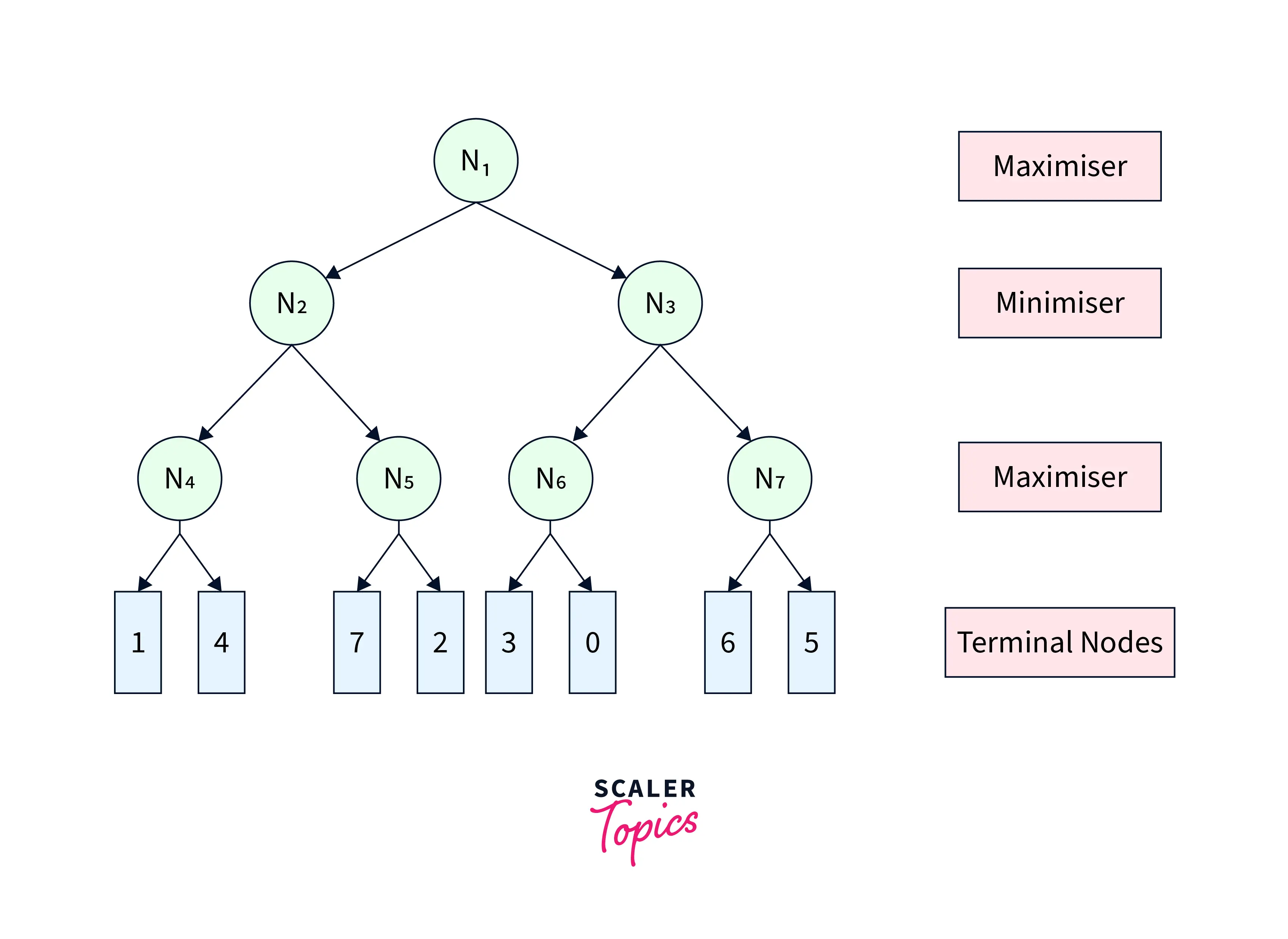Figure-1

The Minimax algorithm would have traversed the complete game tree leading to the game tree shown in Figure-2.

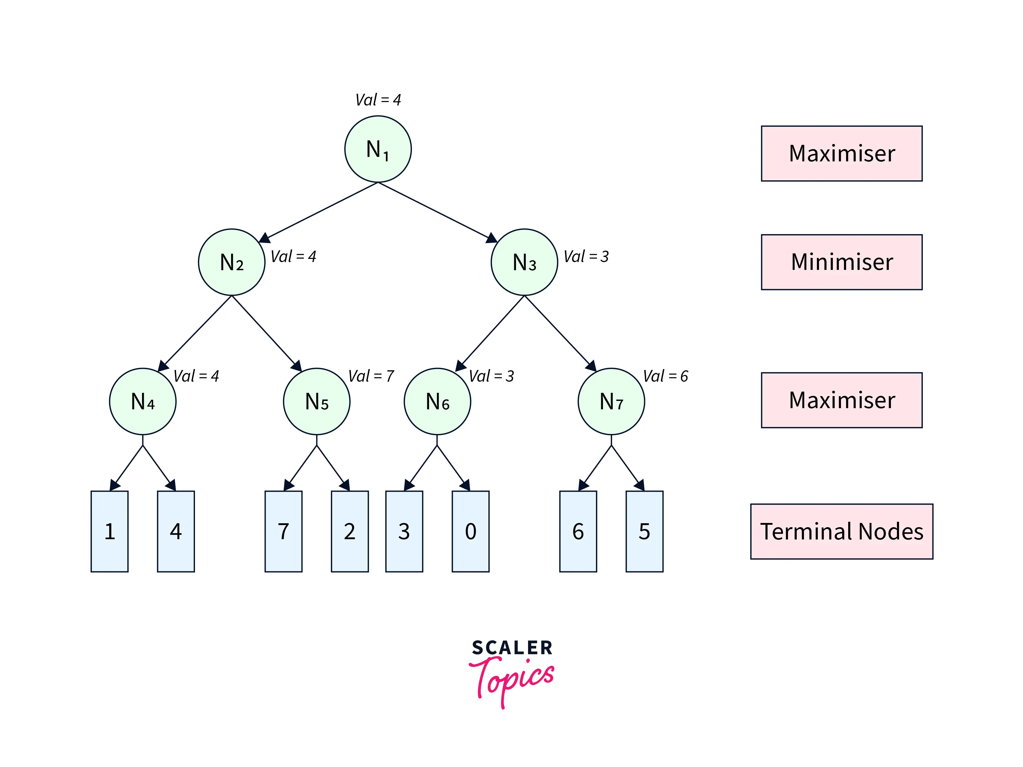Figure-2

Alpha Beta Pruning algorithm restricts the agent from visiting redundant sub-trees leading to faster average search time complexity. To visualize its working, we refer to the same game tree in Figure-1. We start from node $N_1$ with $\alpha=-\infty$ and $\beta=\infty$. From $N_1$, we move to its child node $N_2$ with the same $\alpha$ and $\beta$. Similarly, we move from $N_2$ to its child $N_4$, as shown in Figure-3.

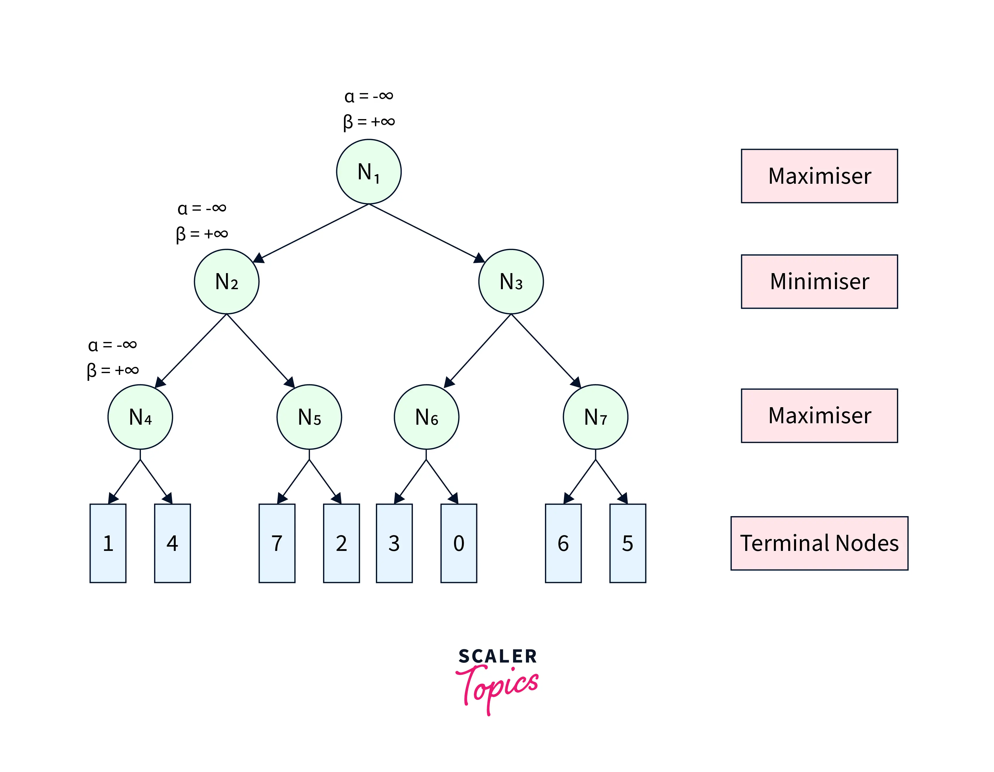Figure-3

From $N_4$, we move to its first terminal child and get back its utility as $1$. Since $N_4$ is a maximiser, we update $\alpha=max(-\infty,1)=1$. The pruning condition $\alpha\geq\beta$ remains unsatisfied. Therefore, we move to the second terminal child of $N_4$ and get its utility as $4$. Further, we update $\alpha=max(1,4)=4$. After this step, we get the node value of $N_4$ as $max(1,4)=4$ and return it to its parent $N_2$. Since $N_2$ is a minimiser, it updates $\beta=min(+\infty,4)=4$. The game tree after this step is shown in Figure-4.

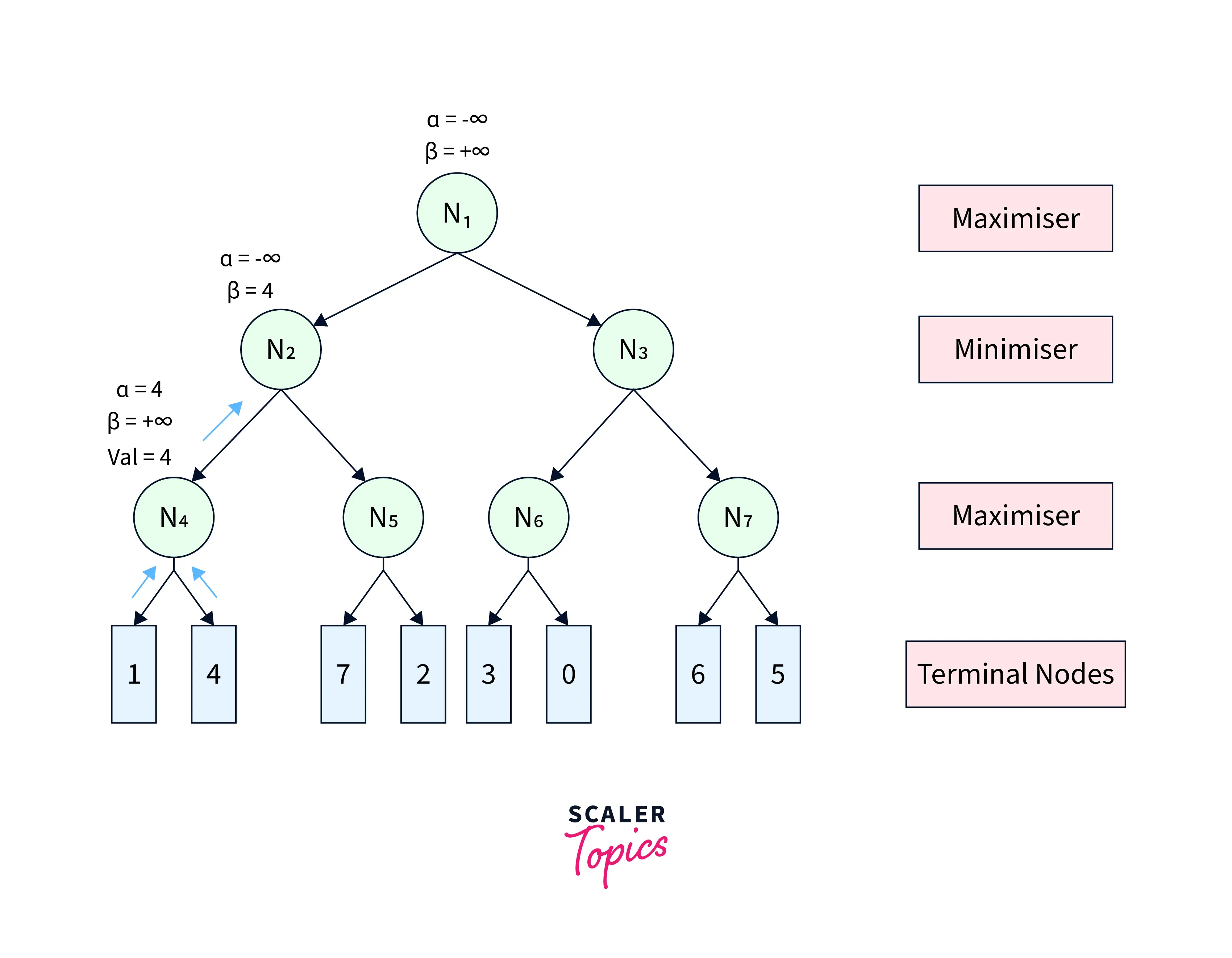Figure-4

At $N_2$, the pruning condition $\alpha\geq\beta$ is still unsatisfied. Therefore, we visit its next child node $N_5$ with $\alpha=-\infty$ and $\beta=4$. At $N_5$, we get the utility of its first terminal child as $7$. Since $N_5$ is a maximiser, we update $\alpha=max(-\infty,7)=7$. Now, the pruning condition gets satisfied $(7\geq4)$, leading to the pruning of the other child node. After that, the node utility of $N_5=7$ is further sent back to the parent node $N_2$. $N_2$ updates $\beta=min(4,7)=4$. Further, the node value of $N_2=min(4,7)=4$ is returned to its parent $N_1$. At $N_1$, we update $\alpha=max(-\infty,4)=4$. After this step, the game tree looks like Figure-5.

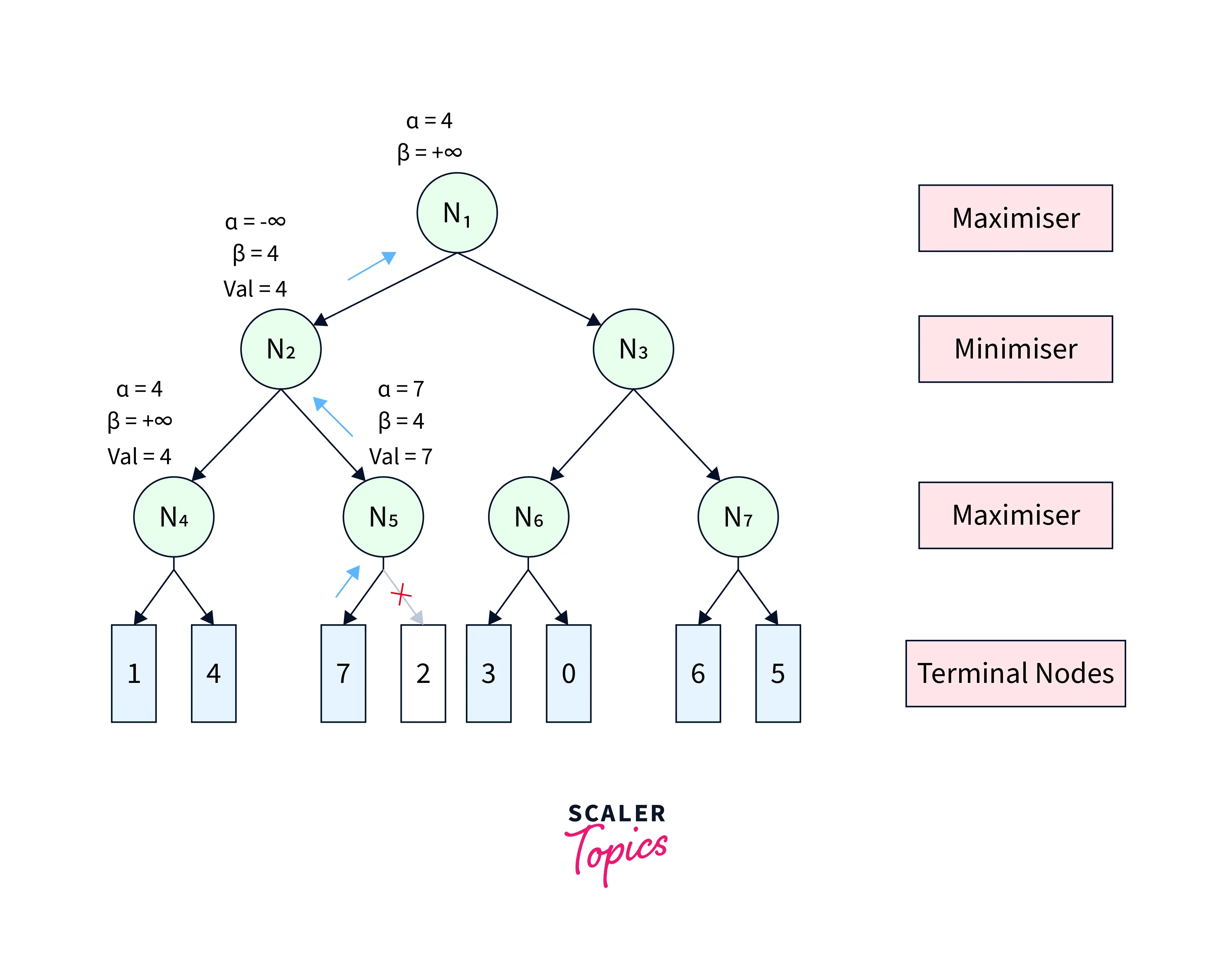Figure-5

The pruning condition is still unsatisfactory at $N_1$. Therefore, we continue towards the next child $N_3$, with the same values of $\alpha$ and $\beta$. Similarly, we propagate from $N_3$ to its first child $N_6$. At $N_6$, we get back the utility of its first terminal child as $3$ and update $\alpha=max(4,3)=4$. Since the pruning condition is still unsatisfied, we get the utility of the second terminal child as $0$ and update $\alpha=max(4,0)=4$. After this, the node value of $N_6=max(3,0)=3$, is returned to the parent $N_3$. Since $N_3$ is a minimiser, we update $\beta=min(+\infty,3)=3$. Now, the pruning condition gets satisfied $(4\geq3)$. Therefore, the other child sub-tree(rooted at $N_7$) of $N_3$ is pruned, and the node value of $N_3$ becomes $3$, which is returned to parent $N_1$. At $N_1$, we again update $\alpha=max(4,3)=4$ and the final utility of $N_1$ becomes $4$. All these steps are shown in Figure-6.

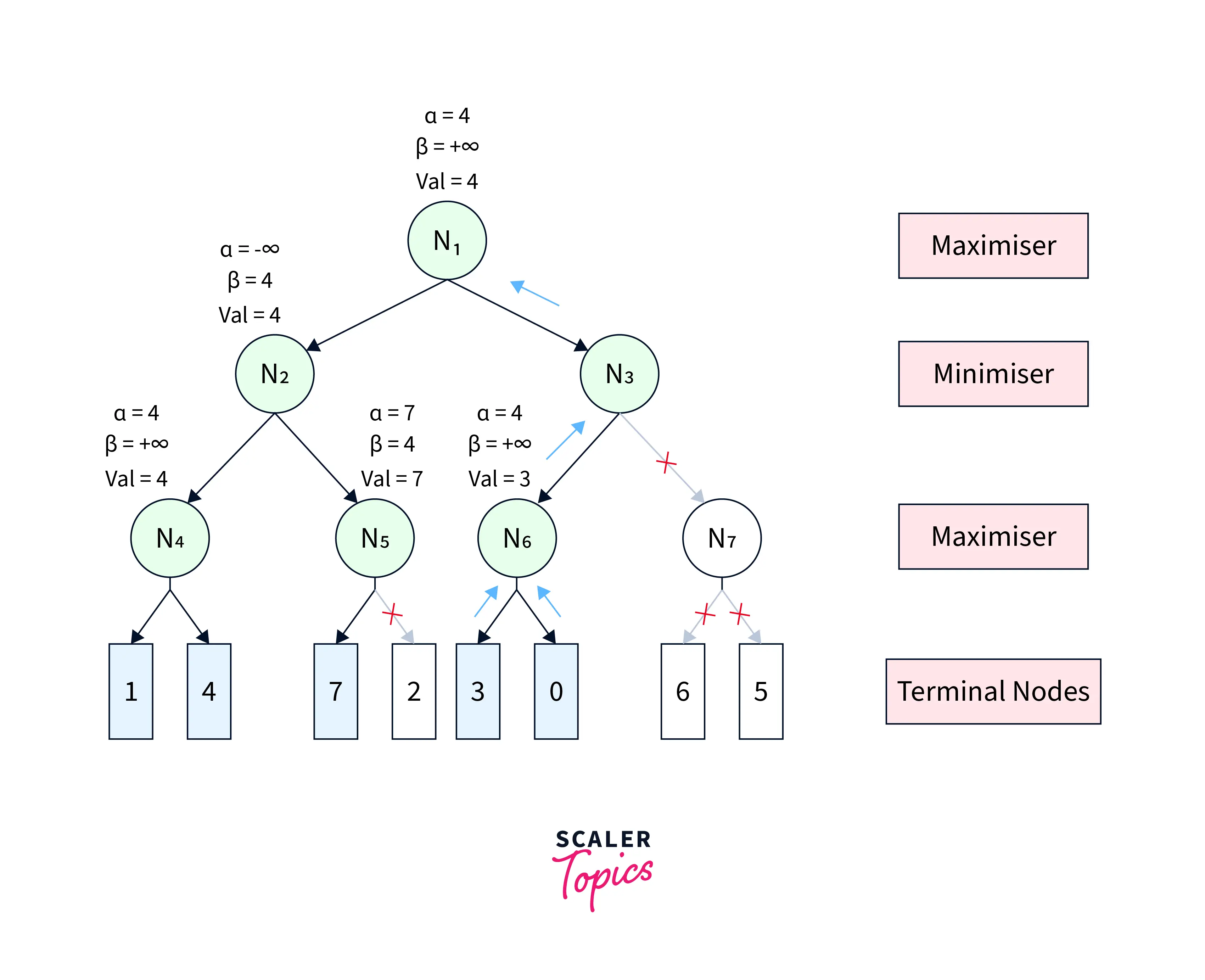Figure-6

Figure-6 depicts the final game tree of the Alpha Beta Pruning algorithm. As evident from the figure, Alpha Beta Pruning in AI yields the same result as the Minimax algorithm by visiting fewer states.

Move Ordering in Alpha Beta pruning in AI

The performance of the Alpha Beta Pruning algorithm is highly dependent on the order in which the nodes are traversed. For instance,

Case-1(Worst Performance): If the best sequence of actions is on the right of the game tree, then there will be no pruning, and all the nodes will be traversed, leading to even worse performance than the Minimax algorithm because of the overhead of computing $\alpha$ and $\beta$. An example game tree can be seen in Figure-7.

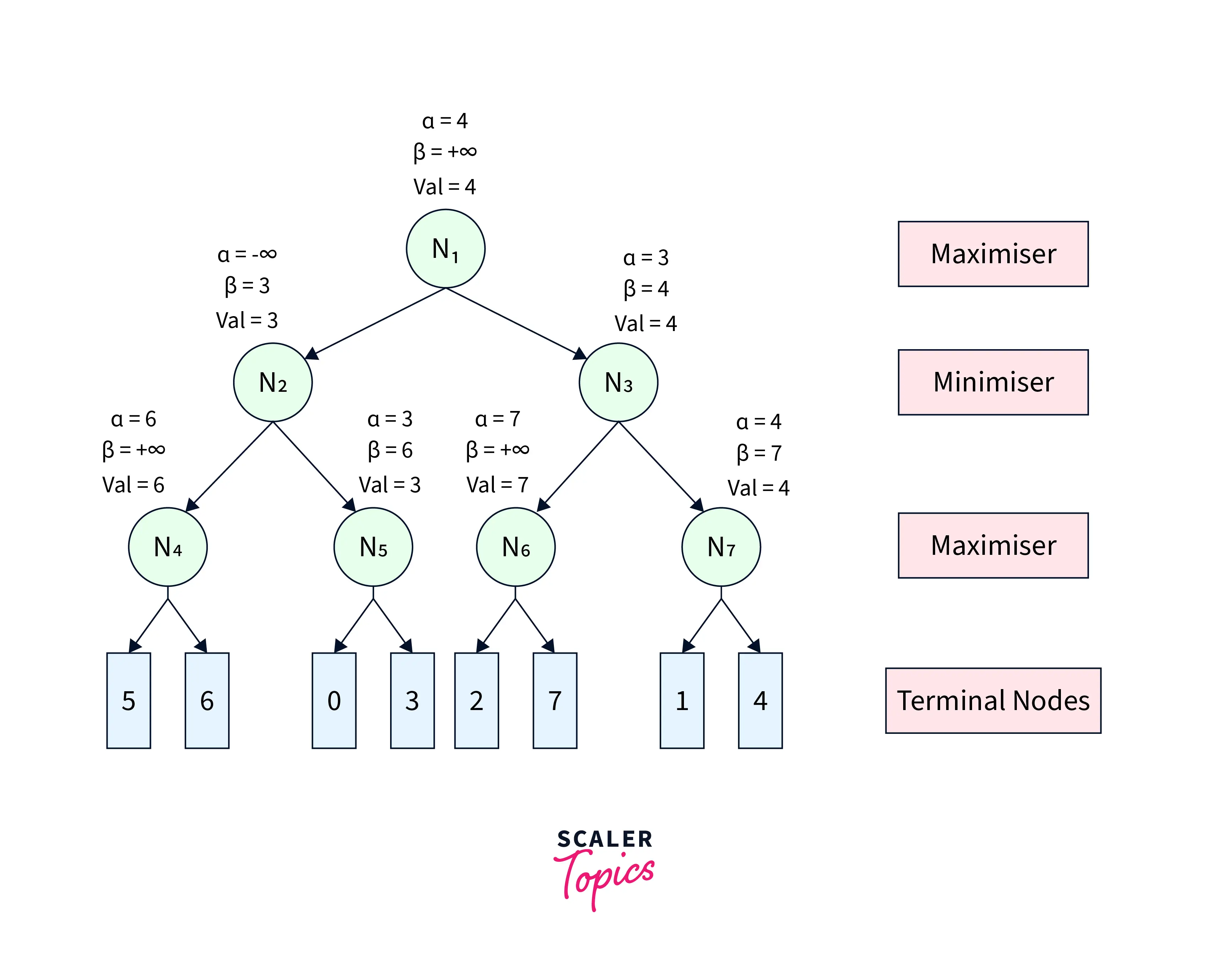Figure-7

Case-2(Best Performance): If the best sequence of actions is on the left of the game tree, there will be a lot of pruning, and only about half of the nodes will be traversed to get the optimal result. An example game tree can be seen in Figure-8.

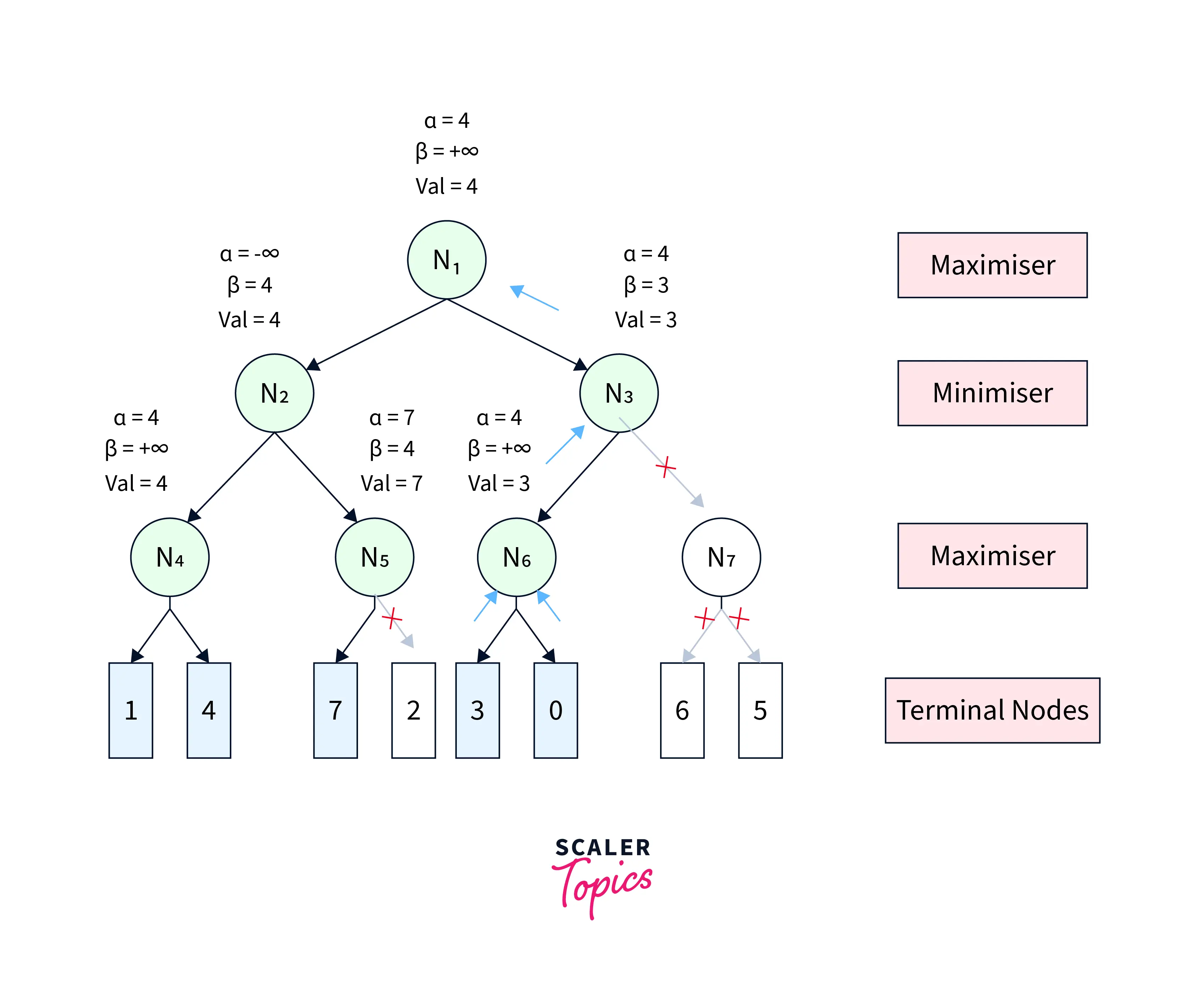Figure-8

Rules to Find Good Ordering

• The best move occurs from the shallowest node.
• The game tree is ordered so that the best nodes are checked first.
• Domain knowledge is used to find the best move.
• Memoization is applied to prevent recomputation in case of repeating states.