Hidden Markov Model
Overview
The Hidden Markov Model in Artificial Intelligence is a framework to statistically represent various systems that are sequential as well as probabilistic in nature. Further, these real-life systems generally have some parameters which are not visible to the ones outside the system. However, these parameters are capable of affecting the visible behavior of the system. Therefore, a Hidden Markov Model exploits this probabilistic relationship between the hidden parameters and the visible observations of a system and helps derive the crucial hidden parameters. As a result, it finds extensive applications in real-life, including Natural Language Processing, Time Series Analysis, and many more.
Introduction
In real life, various processes are sequential in nature and change according to time. Moreover, these changes are not entirely deterministic and can be associated with some probabilities. The Hidden Markov Model in Artificial Intelligence is a mathematical technique for modeling such sequential and stochastic processes and identifying the probabilistic relationship between its sequence of hidden states and its sequence of observations. Before plunging into the details of the Hidden Markov Model in Artificial Intelligence, we briefly present the Markov Property and the Markov Chain.
Markov Property: It states that the future state of an environment depends only on the present state. In other words, the current state already has information about the past states. Therefore, we can write
where denotes the future state at time step and denotes probability. LHS represents the conditional probability of state provided that the previous states are . RHS indicates the conditional probability of future state provided that the current state is .
Markov Chain (or) Markov Process: A Markov Chain/Process comprises a set of states(that obey the Markov Property) and probabilities of transitioning from one state to the other. We use this for modeling the probability of a sequence of these states. An example Markov Chain can be seen in Figure-1.
Figure-1
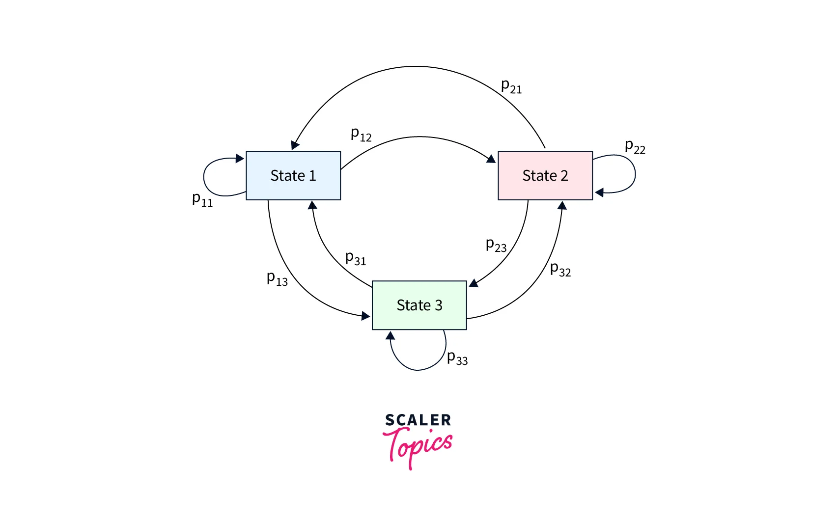
Adding to the complexity of a Markov Chain, a Hidden Markov Model in Artificial Intelligence has some or all of its states as hidden, i.e., we can not see the exact state of the environment. However, the hidden state of the system emits observations with some probabilities. We can use a sequence of these observations to determine the most probable sequence of hidden states the environment has been in. In the next section, we formally define a Hidden Markov Model in Artificial Intelligence.
What is the Hidden Markov Model?
A Hidden Markov Model models a Markov Process with unobservable states using the following components.
- Initial probability distribution of the hidden states denoted as .
- The probabilities of transitioning from one state to another state. This is represented by matrix , where denotes the probability of transitioning from state to state . We call these the transition probabilities.
- The probabilities of obtaining various observations due to a state. This is denoted by the matrix where indicates the likelihood of observation being emitted from state . We also term this as the emission probabilities.
The matrices and constitute the Hidden Markov Model . In line with the Markov Property, the Hidden Markov Model in Artificial Intelligence is based on two assumptions:
- The next hidden state depends only on the current hidden state. Mathematically, we can write
- The observation depends only on the current state. Mathematically, we can write
We can construct the following algorithm to define a Hidden Markov Model in Artificial Intelligence for the concerned problems.
- Step-1: Define the state space and the observation state space of the given problem.
- Step-2: Define the initial probability distribution of the hidden states of the problem.
- Step-3: Define the transition probabilities from one state to the other.
- Step-4: Define the probability of obtaining observations from different hidden states.
- Step-5: After defining all the above parameters of the Hidden Markov Model, train it to find the solution.
- Step-6: Decode the most probable sequence of hidden states from the trained model.
- Step-7: Evaluate the trained model.
The implementation of the above algorithm can be found in the subsequent sections. Now, let us take an example to illustrate Hidden Markov Model in Artificial Intelligence. Bob's mood depends on the weather outside. If the weather is sunny, there is a chance that Bob will be happy and a chance that Bob will be sad. However, if the weather is rainy, Bob will be happy, with a probability of , and sad, with a likelihood of . Bob's friend Alice is sitting inside her house and can not see the weather outside. However, she can observe the mood of her friend Bob and can accordingly guess the weather outside. This situation can be modeled using a Hidden Markov Model where the weather acts as the hidden state and Bob's mood acts as the observation emitted from the hidden states. This can be visualized, as shown in Figure-2.
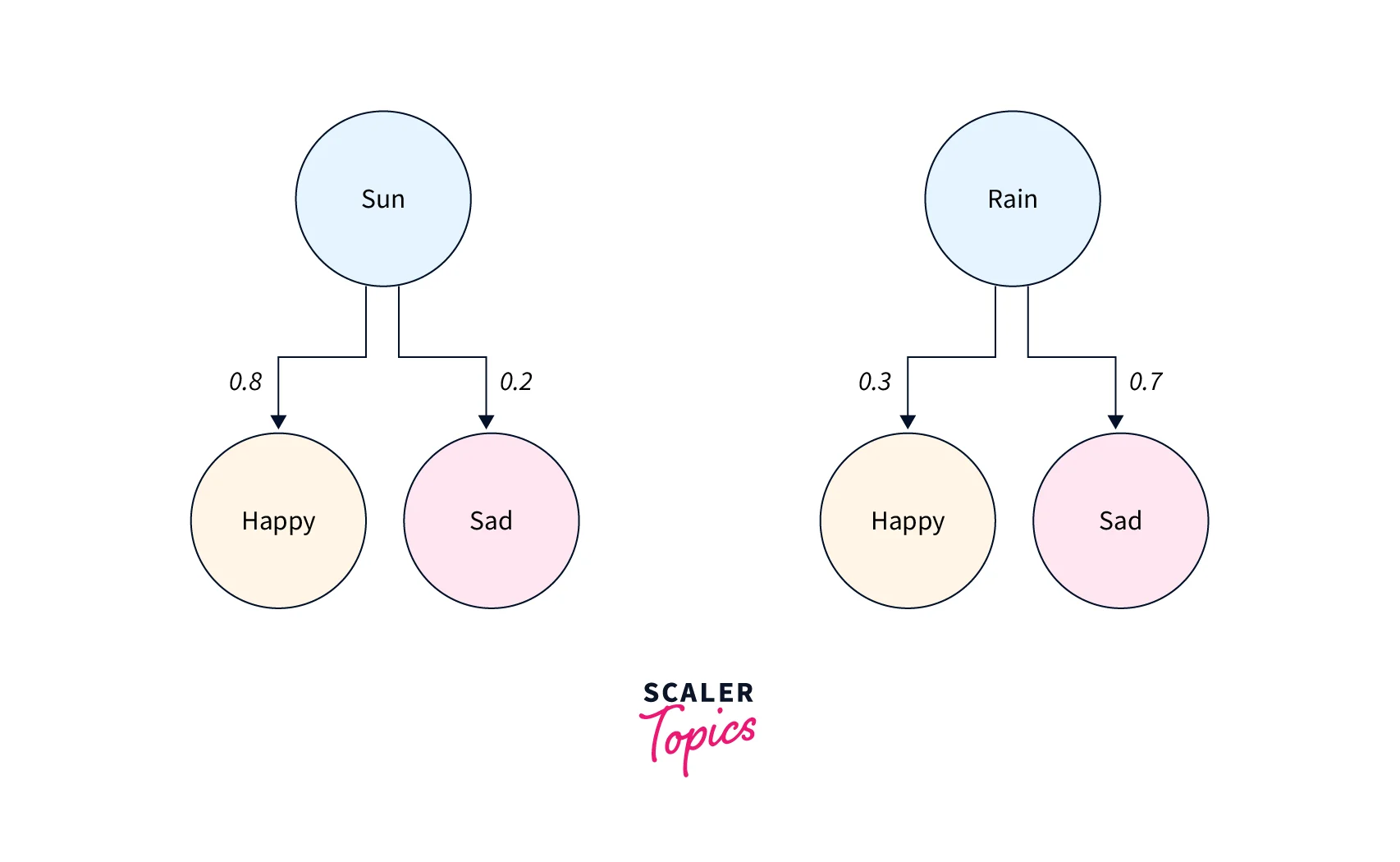
In the next section, we present the various algorithms for solving different components of the Hidden Markov Model in Artificial Intelligence.
Problems to be Solved in a Hidden Markov Model
There are three problems associated with a Hidden Markov Model in Artificial Intelligence, and they are as follows.
- Problem 1 (Likelihood): Given a Hidden Markov Model denoted by and an observation sequence of time steps , we have to determine the probability of the observation sequence, i.e., .
- Problem 2 (Decoding): Given a Hidden Markov Model represented by and an observation sequence of time steps , we have to determine the most probable sequence of hidden states .
- Problem 3 (Learning): Given an observation sequence of time steps and a set of hidden states , we have to learn the parameters and of the Hidden Markov Model while determining the optimal model that maximizes the probability of .
Problem 1 (Likelihood)
There are two algorithms to solve this problem of the Hidden Markov Model in Artificial Intelligence: forward algorithm and backward algorithm. Here, we present the details of the forward algorithm, which is based on dynamic programming. The forward algorithm has three phases: initialization, recursion, and termination.
Initialization
We compute the first forward variable for state by multiplying the likelihood of state and the emission probability of the first observation from the state . Mathematically, we can write the following equation for all hidden states.
Recursion
For computing the forward variable of state, we compute the sum over all the product of forward variable of state, transition probability from state to and the emission probability of observation from state . We can write the following recursive expression for this step.
Termination
After applying the recursive step for time steps, we compute the final desired output by summing forward variable of all states. Therefore, we can write the following expression.
Problem 2 (Decoding)
We use a dynamic programming-based solution called the Viterbi algorithm for this problem. This algorithm also has three phases, namely initialization, recursion, and termination, which are presented below.
Initialization
We compute the first Viterbi variable for the state by multiplying the likelihood of state and the emission probability of the first observation from the state . Mathematically, we can write the following equation for all hidden states.
Recursion
For computing the Viterbi variable of state, we compute the maximum over all the product of Viterbi variable of state, transition probability from state to and the emission probability of observation from state . We can write the following recursive expression for this step.
Termination
After applying the recursive step for time steps, we can figure out the most probable hidden state of time step by selecting the index with the highest Viterbi value . Similarly, for each , we can select the most probable hidden state by choosing the index with the highest Viterbi value . In this manner, we can determine the most probable sequence of hidden states .
Problem-3 (Learning)
This problem can also be solved using a dynamic programming-based approach called Forward-Backward Algorithm or Baum-Welch Algorithm. This comprises four phases, namely initialization, forward phase, backward phase, and update phase. The forward phase involves the following recursive function.
The backward phase is executed using the following recursive function.
For more details on this algorithm, please consult this link.
The following section describes a hands-on implementation of the Hidden Markov Model in Artificial Intelligence using Python.
Implementation of the Hidden Markov Model in Python
We will use Python to implement the Hidden Markov Model of weather-driven Bob's mood presented earlier. In this problem, the weather denotes the hidden state. There are two hidden states, namely Sunny and Rainy. Bob's mood is based on the weather outside. In this problem, Bob's mood is the observation we make. If the weather is Sunny, the probability of Bob being Happy is , and Sad is . On the other hand, if the weather is Rainy, the probability of Bob being Happy is , and Sad is .
Alice is staying inside her home and can not see the weather outside. However, she can observe Bob's mood and guess the most probable weather outside. For Alice, the initial probability of the weather being Sunny is , and Rainy is . Having stated the problem statement, we would model this as a Hidden Markov Model in the subsequent steps.
-
Step-1: Import the required libraries Our script would use numpy, seaborn, matplotlib, and hmmlearn libraries.
-
Step-2: Define the model parameters In this part, we will describe the hidden states, the observations, the initial probability distribution of hidden states, transition probabilities, and emission probabilities.
-
Step-3: Create a Hidden Markov Model instance and feed the model parameters In this step, we would create an instance of the Hidden Markov Model using the hmmlearn library and feed the model parameters defined in the previous step.
-
Step-4: Take an observation sequence and use the Hidden Markov Model instantiated in the previous step for decoding the problem and computing the most probable sequence of hidden states.
The entire script for generating the most probable sequence of hidden states is as follows.
The final output of the above script comes out to be the following.
The observation sequence was (Happy, Sad, Happy, Sad, Sad, Happy). As a result, the most probable hidden state sequence came out to be (Sunny, Rainy, Rainy, Rainy, Rainy, Sunny). In the next section, we describe the application of the Hidden Markov Model in Natural Language Processing.
Hidden Markov Models in NLP
As is evident from the definition of the Hidden Markov Model in Artificial Intelligence, it deals with sequential stochastic data. Examples of such time series data include audio, video, and text data. The analysis of text data is done under the purview of Natural Language Processing. Therefore, Hidden Markov Models in Artificial Intelligence are suitable for application in various tasks of Natural Language Processing. One such task is Part Of Speech Tagging, abbreviated as POS Tagging. In the following sub-section, we describe the details of POS Tagging.
What is POS Tagging?
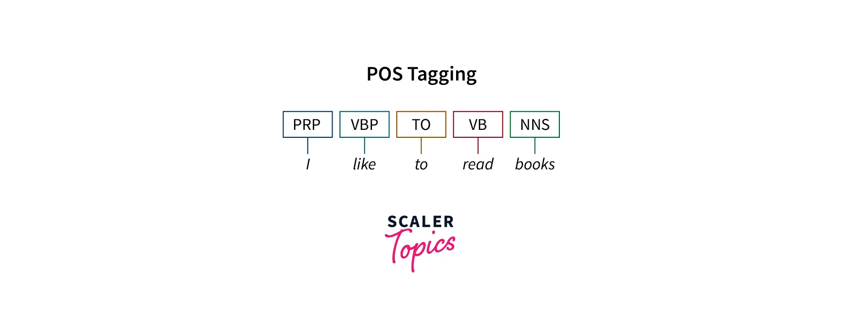
In any English sentence, each word belongs to a specific part of speech. There are commonly used parts of speech in the English Language, namely nouns, pronouns, verbs, adverbs, articles, adjectives, prepositions, conjunctions, and interjections. Now, one of the tasks in Natural Language Processing is POS Tagging, which involves classifying each word in a sentence as one of the nine parts of speech, as shown in Figure-3. In other words, we have to tag each word with its corresponding POS. POS tagging is essential for establishing communication between a machine and a human. One of the most common ways to perform POS Tagging is using the NLTK library in Python. In the next section, we illustrate how we can perform POS Tagging using Hidden Markov Model in Artificial Intelligence.
POS Tagging with Hidden Markov Model
The Hidden Markov Model in Artificial Intelligence is one of the solutions for performing POS Tagging. In this model, the nine parts of speech form the hidden states. Naturally, transition probabilities represent the probabilities of the occurrence of one part of speech after the other. For instance, we need to know the probabilities of the occurrence of a verb after a noun, a noun after an article, and so on. Further, we can not observe the underlying parts of speech, but we can observe the words. Therefore, the emission probabilities would denote the probabilities of the words when the hidden parts of speech are given. As discussed in previous sections, POS Tagging reduces to Problem-2, i.e., decoding the sequence of hidden states(parts of speech) when the observation sequence(sequence of words in the sentence) is given.
For instance, let us say that we have the following corpus of sentences or observation sequences.
- Mary Jane can see Will.
- Will Jane spot Mary?
- The spot will see Mary.
- Mary will pat Spot.
Now, we can build the emission probability matrix as shown below.
| Words | Noun | Modal | Verb |
|---|---|---|---|
| mary | 4/9 | 0 | 0 |
| jane | 2/9 | 0 | 0 |
| will | 1/9 | 3/4 | 0 |
| spot | 2/9 | 0 | 1/4 |
| can | 0 | 1/4 | 0 |
| see | 0 | 0 | 2/4 |
| pat | 0 | 0 | 1/4 |
The word "will" appears time as a noun and times as a modal. Moreover, a noun has appeared times in the corpus, whereas a modal has appeared times. Hence, the emission probability of the observation word "will" when the hidden state part of speech is given as a noun is . Similarly, the emission probability of "will" when a modal is provided as part of speech is . Similarly, we can populate the rest of the matrix. Further, we can construct the transition probability matrix, shown below.
| Noun | Modal | Verb | End | |
|---|---|---|---|---|
| Start | 3/4 | 1/4 | 0 | 0 |
| Noun | 1/9 | 3/9 | 1/9 | 4/9 |
| Model | 1/4 | 0 | 3/4 | 0 |
| Verb | 4/4 | 0 | 0 | 0 |
Here, "Start" and "End" refer to the Start and End tokens added at the ends of each sentence to denote its beginning and end. In the corpus, the Start token appeared times before a noun and time before a modal. Moreover, the Start token appeared times in the corpus. Therefore, the transition probability of the next hidden state part of speech being a noun is when the current hidden state is the Start token. Similarly, the transition probability of the hidden state modal when the current state is a Start token is . Similarly, we can populate the rest of the matrix.
Now, let's take the observation sequence of words "Will Jane spot Mary?". Further, let us take the sequence of hidden states: Start, Modal, Noun, Verb, Noun, and End. We can calculate the likelihood of this sequence by multiplying the respective probabilities shown in Figure-3.
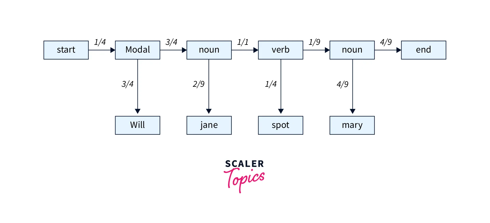
The likelihood of this sequence will come out as
Since the likelihood of the hidden sequence is positive, the sequence of parts of speech is correct. Had it been , we would have concluded that the hidden state sequence is impossible. Therefore, we can have a larger corpus leading to transition and emission probability matrices closer to the real-life scenario. We can accordingly model the problem of POS Tagging as Hidden Markov Model and perform decoding to get the sequence of parts of speech with the highest likelihood. This was a real-life application of the Hidden Markov Model in Artificial Intelligence, and we present more such applications in brief in the next section.
Applications of the Hidden Markov Model
The Hidden Markov Model in Artificial Intelligence has a multitude of real-life applications due to its ability to model stochastic sequential processes while also handling hidden states of the system. Some of those applications are listed as follows.
-
Computational Finance: A Hidden Markov Model can be used to figure out various financial indicators and can help investors adjust their portfolios to maximize their profits.
-
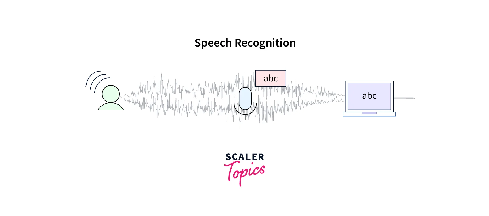
Speech Recognition: Given sequential time-series audio data, a Hidden Markov Model can be used to identify the most probable sequence of underlying words leading to speech recognition.
-
Speech Synthesis: This involves the creation of the most probable speech audio when a text is given. This is useful in various smart devices used in our day-to-day life.
-
Part of Speech Tagging: This involves figuring out the most likely sequence of parts of speech annotated to each of the words of a sentence.

-
Machine Translation: Given a text in one language, a Hidden Markov Model can be used to translate it into another language.
-
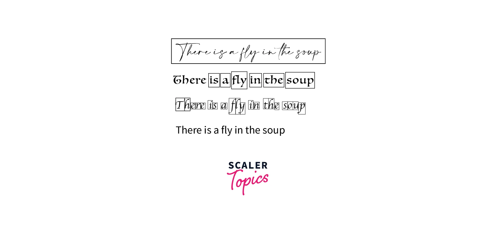
Handwriting Recognition: Given an image of a handwritten text, a machine can use a Hidden Markov Model to figure out the most probable sequence of characters written in the text.
-
Activity Recognition: A Hidden Markov Model can be used to identify the most probable activity from a time-series data stream.
Conclusion
In this article, we learn about the following aspects of a Hidden Markov Model in Artificial Intelligence.
- Definition of Hidden Markov Model along with an example
- The problems of Likelihood, Decoding, and Learning, along with their solutions
- Implementation of a Hidden Markov Model using Python
- Real-life application of the Hidden Markov Model in Part of Speech Tagging in Natural Language Processing
- Various other real-life applications of the Hidden Markov Model in Artificial Intelligence
