Markov Decision Process
Overview
Markov Decision Process(MDP) is a mathematical framework to model sequential decision-making processes in a stochastic environment. This is useful in various real-life applications, including Reinforcement Learning, wherein an agent learns from previous experiences and takes actions accordingly to maximize rewards.
Introduction
In Artificial Intelligence, an agent has to make multiple decisions for choosing the right actions in an environment to gain the highest rewards. Markov Decision Process(MDP) is a mathematical technique to model sequential decision-making processes in a stochastic environment. Before plunging into the details of the main components of Markov Decision Process, we briefly present the concepts of the Markov Property, the Markov Chain, and the Markov Reward Process.
Markov Property:
It states that the future state of an environment depends only on the present state. In other words, the current state already has information about the past states. Therefore, we can write
where denotes the future state at time step and denotes probability. LHS represents the conditional probability of state provided that the previous states are . RHS indicates the conditional probability of future state provided that the current state is .
Markov Chain (or) Markov Process:
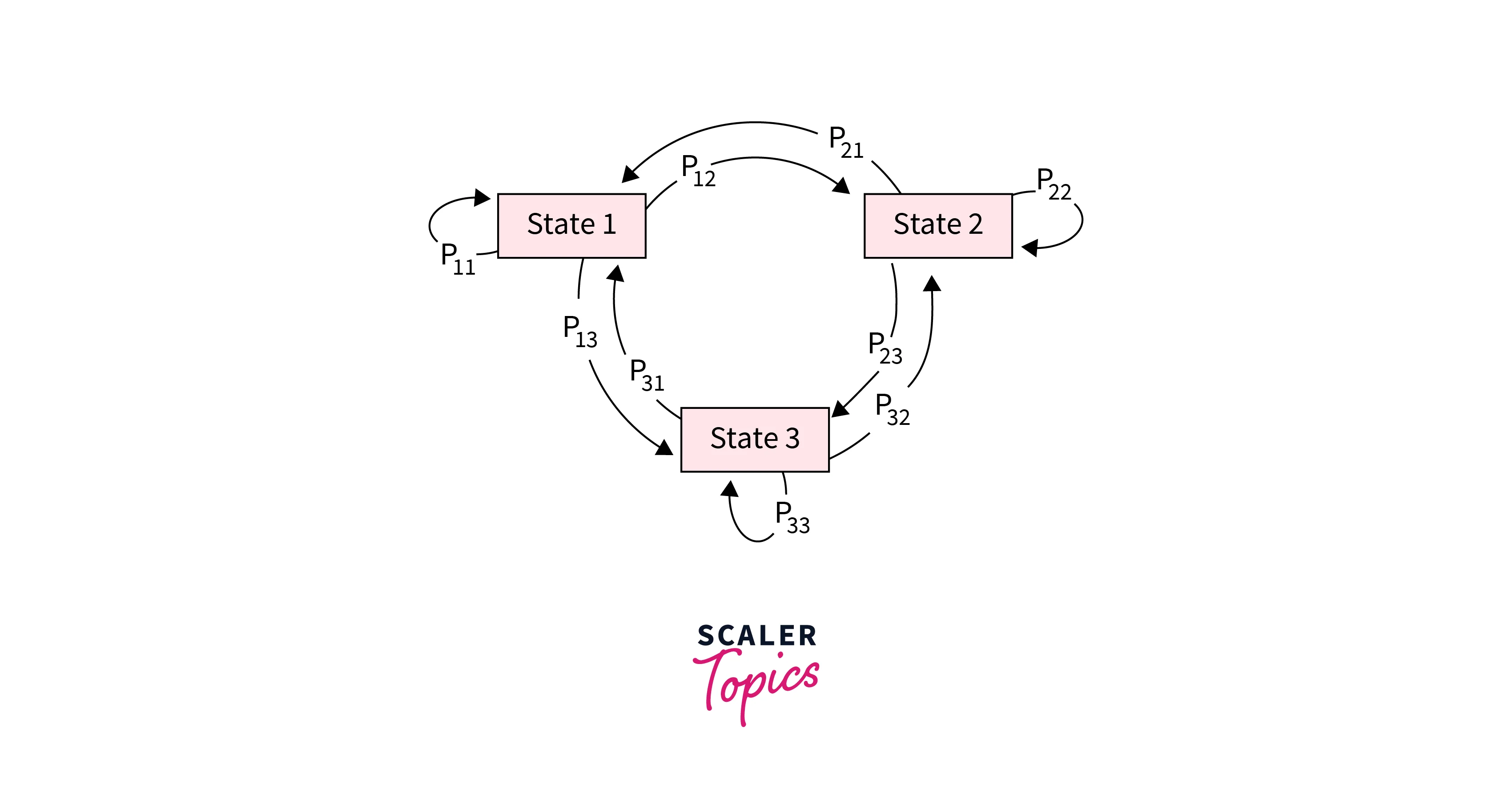
It comprises states that follow the Markov property, and there are some possible transitions between these states. Each transition has a probability associated with it, where denotes the transition probability matrix. A Markov process can be represented as a sequence of states stochastically governed by and . An example can be seen in Figure-1.
Markov Reward Processes:
Adding to the complexity of Markov Chains, we can associate a reward with each state. Further, the Markov Return aggregates rewards collected after a sequence of transitions. However, when there are no terminal states, computing the Markov Return becomes problematic because it becomes possible to keep transitioning amongst the states leading to an infinite sum of rewards. Therefore, we use the concept of discounted future rewards, which multiplies a factor of with the reward obtained after steps in future. Here, refers to the discount factor, which leads to a finite Markov Return value . Therefore, we can write the following expression.
decides the importance that needs to be given to future rewards. For a large , future rewards are given higher weightage, whereas for smaller , immediate rewards are preferred.
Markov Reward Process can be defined as where
- denotes the set of states.
- means the transition probability matrix.
- refers to the reward function, which assigns a reward to each state.
- represents the damping factor.
Markov Decision Process is a Markov Reward Process with an agent that takes decisions to choose amongst the possible transitions. In the next section, we present the formal definition of the Markov Decision Process and its working.
What is the Markov Decision Process?
Mathematical Definition
A Markov Decision Process can be represented by the tuple where
- refers to the set of states in the environment.
- denotes the set of possible actions that the agent can choose.
- represents the probability distribution of the next state when the current state and chosen action are given.
- refers to the reward the agent obtains after choosing an action at its current state.
- refers to the discount factor used to compute discounted future rewards.
In the following sub-section, we describe the main components of Markov Decision Process and their working.
Working of Markov Decision Process
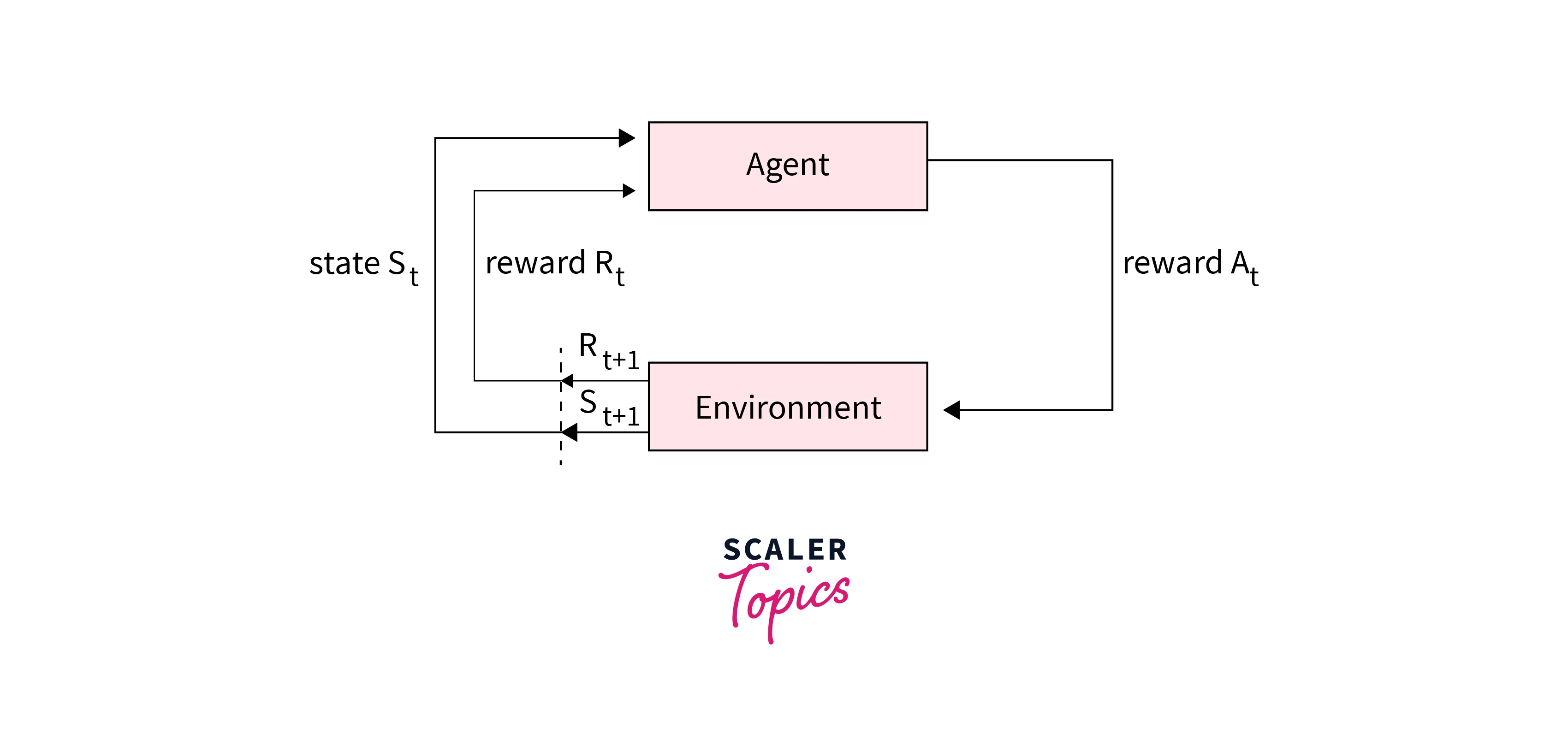
Initially, the environment is in some state . The agent chooses an action and performs it. As a result, the environment changes its state to with a probability given by . Subsequently, the agent receives a reward , which is the expected reward, given the state and the chosen action. This mechanism is reiterated at the state . These main components of Markov Decision Process are illustrated in Figure-2.
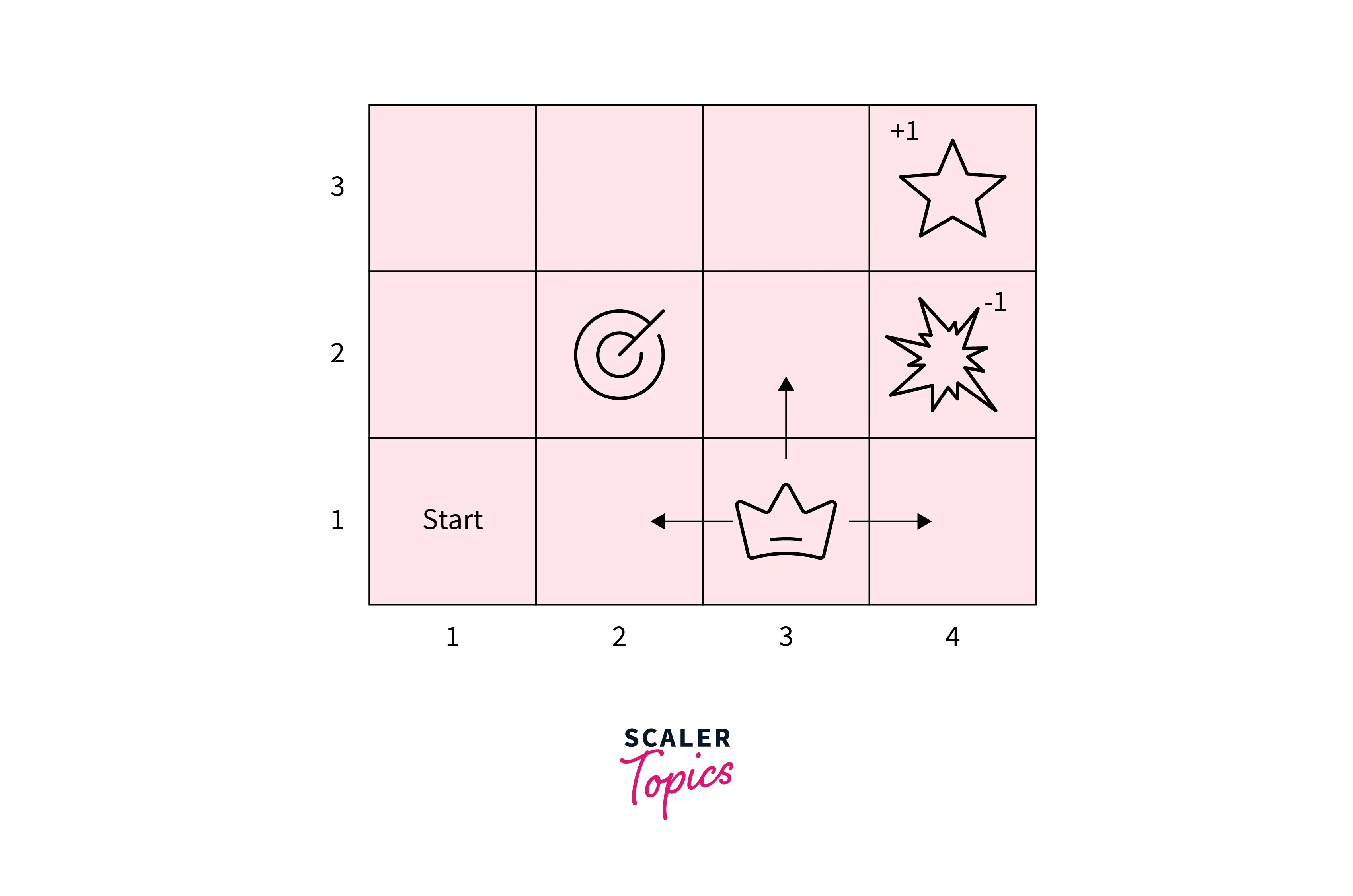
Let us take an example of a Markov Decision Process. There is a grid of size which acts as our environment. The cell represents the START state where the agent stands. The agent's task is to wander in the grid and find the diamond to get a reward of . Naturally, the position of the diamond on the grid is unknown to the agent.
Further, some cells have a fire where the agent gets a reward of on stepping. Some cells are blocked and can not be traversed by the agent. The agent can move UP, DOWN, LEFT and RIGHT in four directions. However, the movement is stochastic. There is an chance that the movement will be in the intended direction and a chance that it will happen in a perpendicular direction. This setup is shown in Figure-3.
Now, we can model the main components of Markov Decision Process as follows:
- Each cell represents a state leading to a total of states.
- There are four possible directions of movement for the agent, namely UP, DOWN, LEFT and RIGHT. Therefore, these four directions are the set of possible actions for the agent. However, not all actions are possible at boundary cells.
- Since the movements are stochastic, there will be a probability distribution of the next state when the current state and chosen action are given. For example, if the current state is and the chosen action is UP, then the probability of the next state being will be , will be and will be .
- The fire and the diamond cell(state) have their associated reward as and , respectively. The other cells have a reward. Therefore, for each state and action, we can write the reward function as the weighted sum of rewards of the possible next cells. Weights refer to the respective transition probabilities.
- This can be any number between and . Generally, the values are taken between and .
The agent's goal is to maximize its cumulative sum of rewards. Therefore, it needs to choose its actions optimally. In the next section, we will look at two primary components of the Markov Decision Process, i.e., policy and value function, which help the agent choose the optimal actions to gain maximum rewards.
Policy and Value Function of Markov Decision Process
A policy of a Markov Decision Process is a function that takes a state as an input and outputs the action that the agent following that policy should choose. In other words, it is a mapping between states and actions. As a result of this mapping, different policies can lead to varying amounts of cumulative rewards. Now, the goal of an agent is to maximize the cumulative rewards. Therefore, the agent must choose a policy that leads to the same. Such a policy is known as an optimal policy. Further, to search for an optimal policy, we use discounted future rewards due to reasons discussed previously.
The value function of a Markov Decision Process takes a state as input and outputs the expected cumulative rewards if the agent starts at that state and follows a particular policy. Therefore, we can write the following expression.
The value function can be broken down into the reward generated after choosing an action at the current state and the expected cumulative rewards at the next state. This leads to the Bellman equation, which is stated as
is the value function that returns the maximum possible cumulative reward at a particular state. This can be achieved when an optimal policy is used. Therefore, we can write the expression for the optimal policy as
There are various algorithms to compute the optimal policy and value function of a Markov Decision Process. Optimal value function can be computed using multiple iterative methods such as Monte Carlo evaluations, Dynamic Programming, Temporal Difference learning and many more. Optimal policy functions can be computed using policy iteration, Q-learning, value iteration, and linear programming. In the next section, we present the various applications of the Markov Decision Process.
Applications of Markov Decision Process
Routing problems
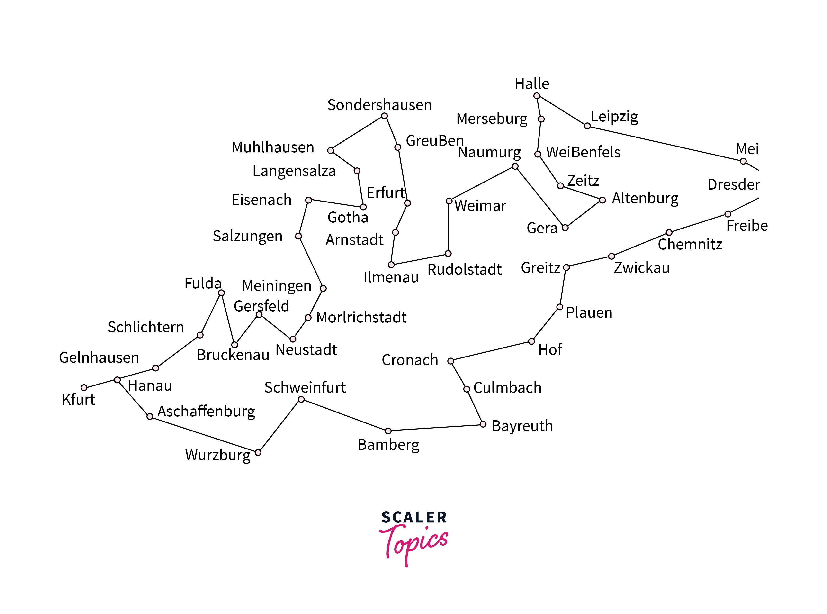
Travelling Salesman Problem is a renowned routing problem that involves sequential decision-making and can be addressed by the main components of Markov Decision Process. The salesman becomes the agent, and the available routes become the set of actions. Rewards can be specified as the cost of traversing the routes, and the end goal is to search for an optimal policy that minimizes the cost for the entire duration of the trip. An example solution of the Travelling Salesman Problem over the map of France is shown in Figure.
Maintenance and Repair of Dynamic Systems
Dynamic systems include various machines that operate in varied conditions, like cars, buses, trucks, and many more. These systems need time-to-time maintenance. Therefore, the possible actions can be ignoring maintenance, performing maintenance, replacing critical parts and many more. These actions can be taken by observing the state of the dynamic system. The goal is to minimize the maintenance and repair costs over the long run while keeping the system functional. As is evident from the problem structure, this can be solved using Markov Decision Process.
Designing Intelligent Machines
Markov Decision Process is extensively used in association with advanced Machine Learning and Artificial Intelligence frameworks. Some applications of this kind include robotics, complex autonomous systems, autonomous vehicles, and many more.
For example, Google's subsidiary, DeepMind Technologies, combines the main components of Markov Decision Process with Neural Networks for training systems to play games like Atari, AlphaGo etc., even better than humans. Markov Decision Process is also used to teach robots various motion actions like walking and running.

Designing Quiz Games
Markov Decision Process is highly used in quiz games. In such games, the agent has to answer a question for each level. If the agent answers correctly, it advances to the next level, which has a question of greater difficulty. If the agent answers all questions of the game correctly, then it receives a reward. Further, the agent can either quit the game or replay it. While replaying, if the user gives a wrong answer, then the accumulated rewards are lost. Therefore, there is a tradeoff between quitting the game with lesser risk and replaying the game with a higher risk. The agent aims to evaluate these two actions and choose the optimal one while maximizing the gained rewards.
Managing Wait Time at a Traffic Intersection
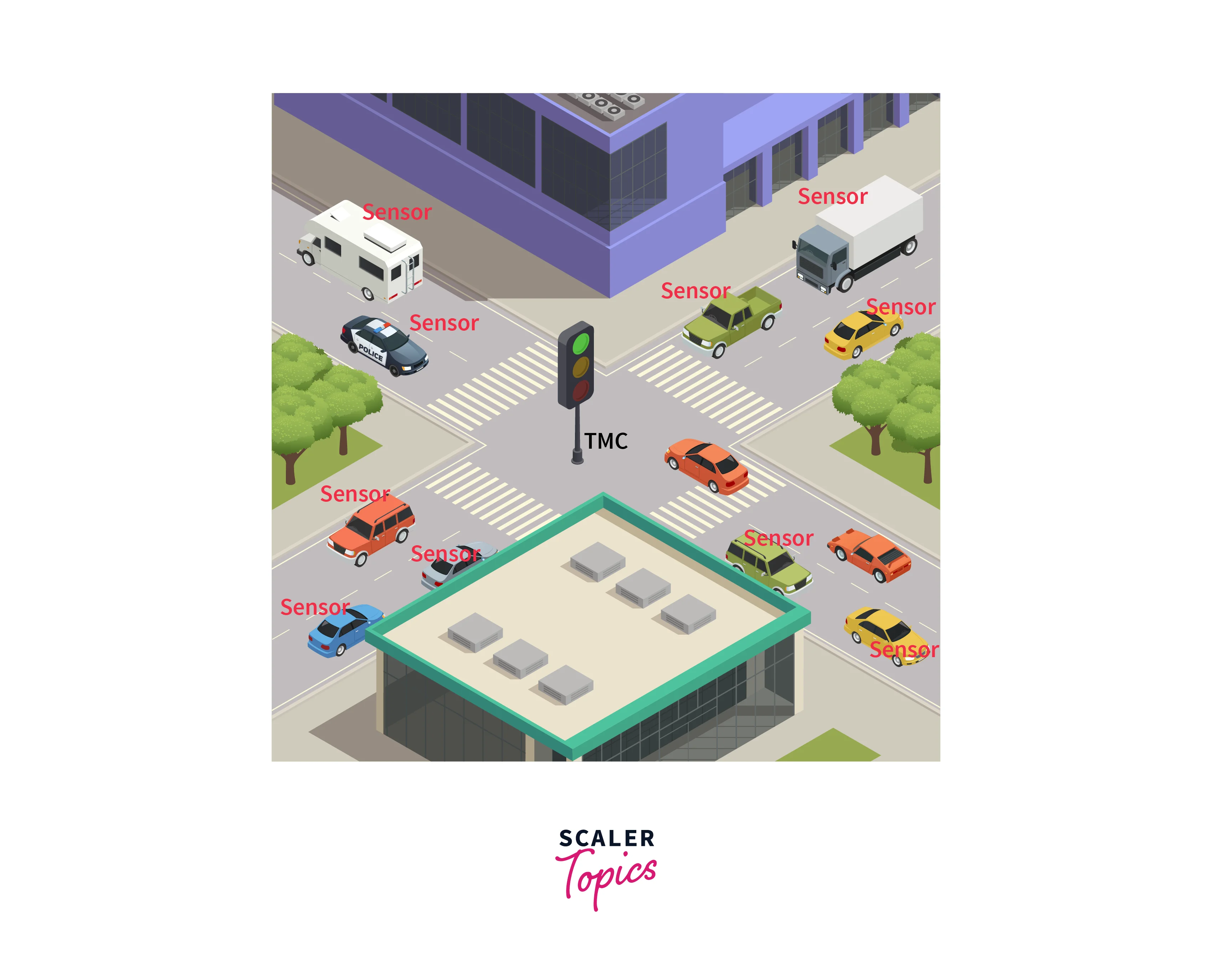
The duration of traffic lights being red or green can also be modelled by the main components of Markov Decision Process. The goal is to maximize the flow of traffic vehicles through a junction while also checking their waiting times. This setup needs data on the number of traffic vehicles approaching a junction. Each step takes a few seconds, and the two states of the system are red and green. By solving this Markov Decision Process, we can decide if we need to change the signal depending on the number of traffic vehicles passing through the junction and waiting times.
Determining the Number of Patients to Admit to a Hospital
A hospital has to decide the number of patients to be admitted based on various factors like the number of available beds, number of already admitted patients, number of patients recovering and getting discharged daily, and many more. The hospital's objective is to determine the number of patients that can be admitted while maximizing the number of patients recovering over a period of time. This can also be modeled using the main components of Markov Decision Process.
Likewise, there are numerous applications of the Markov Decision Process. In the next section, we discuss the utility of the Markov Decision Process in Reinforcement Learning.
Utility of Markov Decision Process in Reinforcement Learning
In Reinforcement Learning, an agent makes decisions to choose amongst possible actions and learns from past experiences. After selecting an action, the environment provides a reward to the agent. This reward can be positive as well as negative. Negative rewards can be seen as a punishment. Naturally, the goal of the agent is to maximize the cumulative rewards. In such a scenario, the agent faces the dilemma of exploitation vs exploration. A strictly exploitative agent depends only upon previous experience to maximize its rewards. On the other hand, a purely explorative agent ignores its experiences and keeps on finding better ways to gain higher rewards. Therefore, a purely exploitative agent might miss out on higher rewards, whereas a strictly explorative agent might have a very high search cost.
Practically, we need a mixture of both characteristics in an agent. Therefore, the agent is generally set to be more explorative initially and then become more exploitative in the later phases. We use Markov Decision Process to model such a situation mathematically. We can define the main components of Markov Decision Process and compute the optimal policy for an agent by using various algorithms like Q Learning etc. Hence, Markov Decision Process is highly crucial in modeling Reinforcement Learning problems.
Conclusion
In this article, we discussed
- A brief illustration of Markov Property, Markov Chains and Markov Reward Process.
- Mathematical definition of Markov Decision Process and its working
- Policy and Value function of a Markov Decision Process
- Applications of the Markov Decision Process along with its utility in Reinforcement Learning
