Partially Observable Markov Decision Processes (POMDPs)

Pre-requisites

• Concepts of conditional probability
• Markov Decision Processes
• Basic Programming knowledge

Introduction

In Artificial Intelligence, an agent/decision-maker needs to go through various decision-making processes to take appropriate actions in an environment to maximize the gain of rewards. Partially Observable Markov Decision Process (POMDP) is a mathematical framework to model sequential decision-making processes in real-life scenarios wherein the decision-maker does not have complete information about the environment in which it works. Therefore, POMDP finds its applications in various domains like AI, operations research, economics, robotics, and many others. We formally define POMDP in the next section.

What are POMDPs?

A POMDP can be represented by the tuple $(S, A, T, R, \Omega, O, \gamma)$ where,

• $S:$ refers to the set of states in the environment.
• $A:$ denotes the set of possible actions taken by the decision maker.
• $T:$ refers to a conditional transition probability distribution of the next state when the current state and chosen action are given.
• $R:$ is a function that takes state and action as input and provides the corresponding reward as output.
• $\Omega:$ refers to the set of possible observations made by the decision-maker.
• $O:$ is a conditional probability distribution of the observations when the current state and chosen action are given.
• $\gamma:$ represents the discount factor used to compute the expected sum of discounted future rewards.

Initially, the environment is in some state $s \in S$. The decision maker chooses an action $a \in A$ leading to the transition of the environment to the next state $s' \in S$ with the conditional probability given by $T(s' \vert s, a)$. However, unlike Markov Decision Process (MDP), the decision maker can not know about the actual state of the environment but can only make some observations. Therefore, the decision maker makes an observation $o \in \Omega$. Further, the observation $o$ depends on the new state $s'$ and the chosen action $a$ with the conditional probability $O(o \vert s', a)$. Ultimately, the decision maker receives a reward denoted by $R(s, a)$. This entire process is repeated for multiple iterations, leading to a sequence of decisions of actions the decision maker takes.

Given the above framework, the goal of the decision maker, in a similar fashion as the Markov Decision Process (MDP), is to maximize the expected sum of discounted future rewards denoted by $E[\sum_{t=0}^{\infty}\gamma^{t}r_{t}]$ where $r_{t}$ indicates the reward obtained at time step $t$. Now, let us take a simple example of a problem that can be formulated as a POMDP.

Suppose there is a robot that can move in a $3 \times 3$ grid environment. At each time step, the robot can take one of four actions: move up, move down, move left, or move right. However, the robot's movements are not entirely deterministic. If it tries to move in a specific direction, it has a 70% chance of succeeding and a 30% chance of moving in a random direction. The robot also has a sensor that can detect whether it is in the top row, middle row, or bottom row of the grid world. However, the sensor is not entirely reliable. It has an 80% chance of giving the correct reading and a 20% chance of giving a random reading.

The goal of the robot is to navigate to a particular cell (denoted as the "target cell") in the grid world. However, the robot doesn't know the location of the target cell initially. It only knows that it is in one of the nine cells in the grid world. At each time step, the robot can take action to move and observe the sensor reading, and based on this information, it must decide what action to take next to maximize its chances of reaching the target cell.

This problem can be formulated as a POMDP, where the state of the system is the robot's location (unknown to the robot), and the belief state is a probability distribution over the possible locations of the target cell. The observation is the reading from the sensor, and the action is the robot's movement. The objective is to find a policy that maximizes the expected cumulative reward, which could be defined as the negative Manhattan distance between the robot's current location and the target cell. This example is a simplified version of a classic problem in robotics called the "grid localization" problem, which is often used as a benchmark for testing POMDP algorithms.

Solving POMDPs

Formulation of POMDP as Belief State MDP

Let us define $b$ as belief which is a probability distribution of states that the decision maker thinks the environment might be in. In other words, for a state $s$, $b(s)$ represents the probability/belief of the decision maker that the environment is in state $s$. After choosing an action $a$ and making the observation $o$, the decision maker needs to update the belief to $b'$. Assuming that belief follows the Markovian property, i.e., the current belief state depends only on the previous belief state, we can write $b'$ as a function of $b$, $a$, and $o$. Therefore, we can write $b' = \tau(b, a, o)$.

Now, once the decision maker chooses action $a$ and makes observation $o$ with the current belief of a state $s$ being $b(s)$, we can write the updated belief of a state $s'$ as

where,

$\eta = 1/\text{Pr}(o \vert b, a)$ and $\text{Pr}(o \vert b, a) = \sum_{s' \in S} O(o \vert s', a) \sum_{s \in S} T(s' \vert s, a)b(s)$.

Informally stating for intuition, we first get the probability that the environment was in state $s$ by $b(s)$. Further, we get the conditional probability of the current state being $s'$ provided that the previous state and chosen action were $s$ and $a$, respectively. However, we want to encompass all cases when transitioning to the state $s'$. Therefore, we do this operation using a summation for all possible previous states. Furthermore, we compute the probability that the state $s'$ and chosen action $a$ lead to observation $o$. Lastly, to calculate the probability/belief of $s'$, we also need to divide it by the summation of values about each possible current state $s'$.

Now, we can formulate POMDP as a belief state MDP which can be defined as the tuple $(B, A, \tau, r, \gamma)$ where

• $B:$ is the set of belief states.
• $A:$ corresponds to the set of actions of the original POMDP.
• $\tau:$ denotes the transition function, which takes the current belief and chosen action as input and renders the new belief state as output.
• $r:$ is the reward function that takes the current belief and chosen action as input and generates the corresponding reward.
• $\gamma:$ refers to the same discount factor used in the original POMDP.

Before proceeding, we must define $\tau$ and $r$ in terms of the original POMDP. We can write

$\tau(b, a, b') = \sum_{o \in \Omega} \text{Pr}(b' \vert b, a, o)\text{Pr}(o \vert a, b)$

The value of $\text{Pr}(b' \vert b, a, o)$ will be $1$ if we get $b'$ after performing the belief update using $b$, $a$, and $o$. Otherwise, the value would be $0$. Further, we can define the reward function as

$r(b, a) = \sum_{s \in S} b(s)R(s,a)$

The intuition behind these formulations can be derived similarly to the one behind the belief update formula. One crucial observation to be made here is that the belief MDP has a continuous state space, unlike the original POMDP, which had discrete states. The reason is that the belief states are probability distributions that can take any values between $0$ and $1$. In the subsequent sub-sections, we present the techniques to solve the belief MDP and hence the POMDP as well.

Exact Value Iteration

Before proceeding to the algorithm, we need to define the notation $V^{k}(s_{i})$ as the maximum possible expected sum of discounted future rewards if the decision maker takes decisions for $k$ time steps and starts from state $s_i$ in the case of a discrete MDP. Further, we write $V^{1}(s_i) = r(s_i) =$ reward gained at state $s_i$. To compute $V^{k}(s_{i})$, we can make use of $V^{k-1}(s_{i})$ by the following equation

Now, as $k \rightarrow \infty$, we get $V^{*}(s_{i})$, which is the value function and is a solution to the Bellman optimality equation and denotes the maximum possible discounted future reward.

However, in the case of a belief state MDP, we have a continuous state space. Therefore, we need to define value function over our continuous belief state space. We can write

Now, if we plot this value function against the state utilities, then we get a piecewise linear convex graph. In other words, the value function of POMDPs can be represented as the maximum of linear segments. The linear segments correspond to the various possible actions. For simplicity, if we take two states and two actions, $a1$, and $a2$, then one possible plot of the value function can be as follows.

A crucial point to consider is that Horizon $k$ segments are linear combinations of Horizon $k-1$ segments. Horizon $k$ refers to the value function obtained after $k$ iterations. Therefore, the value iteration algorithm can be broadly stated as follows

1. Calculate value function vectors for each action
2. Transform value function with observations
3. Repeat steps 1 and 2 for the next horizon value function until convergence

Exact Value Iteration is an exact algorithm to find the optimal solution of POMDP. However, the time complexity is exponential, and the belief dimensionality increases with the number of states.

Policy Iteration

Let us define $V^{\pi}(b)$ as the expected discounted future reward following policy $\pi$ from belief state $b$ in a discrete MDP. A policy tells us about the action that should be chosen when the decision maker is in a particular state. Now, a policy $\pi^*$ is an optimal policy if it yields the maximum expected discounted future reward.

Therefore, our goal is to find an optimal policy that can be done using policy iteration. The policy iteration algorithm can be stated as follows:

1. Initialise a policy $\pi^0$.

2. Perform policy evaluation by computing the value function $V^{\pi^{k}}$ and update it using Bellman's equation.

3. Perform policy improvement by

   $\pi^{k+1}(b) = argmax_{a} \bigg[r(b, a) + \gamma \sum_{o \in \Omega} Pr(o \vert b, a)V^{\pi^{k}}(\tau(b, a, o)) \bigg]$

4. Repeat steps 2 and 3 until convergence between $\pi^k$ and $\pi^{k+1}$.

Witness Algorithm

The Witness algorithm finds places where the value function does not remain optimal and operates action-by-action and observation-by-observation to build up value vectors. The algorithm can be broadly described as follows:

1. Start with value vectors at the corners of the graph where the states are known.
2. Define a Bellman's equation-based linear program that finds a point in the belief state space where the value of the function becomes incorrect.
3. Add a new vector which is a linear combination of the segments of the old value function.
4. Iterate until no point is found where the value of the function becomes incorrect.

There are various other solutions to POMDP like HSVI, Greedy solutions like Dual Mode control, Q-MDP, and many others. In the next section, we show a tool available in the R programming language to solve POMDPs through programming.

The Functionality of the "pomdp" Package in R Language

There are two steps while using the pomdp package of the R language in solving a POMDP, and they are as follows:

• Defining the POMDP problem using POMDP()
• Solving the problem defined above by using solve_POMDP()

Defining a POMDP Problem

To define a POMDP problem using POMDP(), we need to pass the elements of the problem as arguments to the function, and they are listed below

• states: Set of states $S$
• actions: Set of actions $A$
• observations: Set of observations $\Omega$
• transition_prob: Conditional transition probabilities of states T(s′\vert s,a)
• observation_prob: Conditional observation probabilities O(o \vert s′,a)
• reward: Reward function R(s, a)
• discount: Discount factor $\gamma \in [0,1]$
• horizon: Number of periods to iterate the POMDP.
• terminal_values: A vector of state utilities at the end of the horizon.
• start: Initial probability distribution $b_0$ over the system states $S$
• max: Denotes whether the POMDP is a maximization or a minimization problem
• name: Assign a name to the POMDP problem

For more details on the input format, please refer to the documentation of POMDP()

Solving a POMDP Problem

To solve a POMDP problem defined using POMDP(), we can use the function solve_POMDP(). This function takes an argument model, which signifies the POMDP model created by POMDP(). Another important argument is the method representing the algorithm to solve the POMDP. The available options for the solving algorithm are grid (default), enum, twopass, witness, and incprune. In the next section, we present a renowned POMDP problem and solve it using pomdp.

The Tiger Problem

The Tiger Problem is a renowned POMDP problem wherein a decision maker stands between two closed doors on the left and right. A tiger is put behind one of the doors with equal probability, and treasure is placed behind the other. Therefore, the problem has two states tiger-left and tiger-right. The decision maker can either listen to the roars of the tiger or can open one of the doors. Therefore, the possible actions are listen, open-left, and open-right. However, the observation capability of the decision-maker is not 100% accurate. Therefore, there is a 15% probability that the decision maker listens and interprets wrongly the side on which the tiger is present. Naturally, if the decision maker opens the door with the tiger, then they will get hurt. Therefore, we assign a reward of -100 in this case. On the other hand, the decision maker will gain a reward of 10 if they choose the door with treasure. Once a door is opened, the tiger is again randomly assigned to one of the doors, and the decision maker gets to choose again.

Now, we formulate this POMDP using the following code

Now, to solve the above Tiger Problem using the default grid method, which uses point-based value iteration, we can execute the following code.

The computed policy for the Tiger Problem can be represented as a graph shown below.

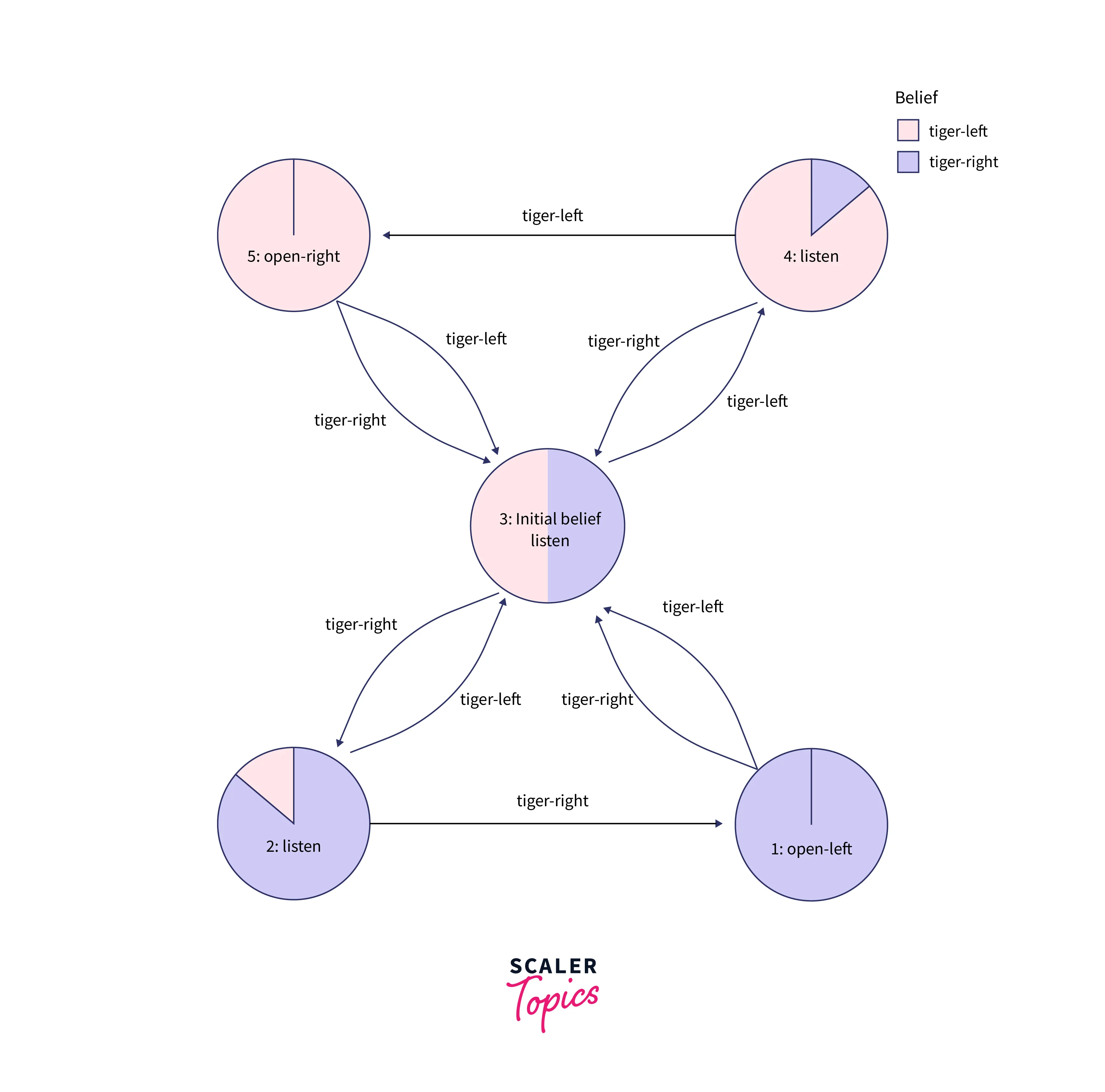
As can be interpreted from the above graph, the decision maker starts at the "Initial Belief" state, wherein there is an equal probability of the tiger being behind the left or right door. Once an observation of "tiger-left" is made, the decision maker again chooses to listen. If the second observation is different, then the decision maker returns to the "Initial Belief" state. However, if the same observation is made twice, the decision maker chooses to open the right door. A similar case happens for the observation "tiger-right". Once the reward is obtained, the problem is reset, and the decision maker returns to the "Initial Belief" state. In the subsequent sections, we present extensions to the POMDP problem and its applications.

Extensions of POMDP

Monte Carlo POMDPs

Monte Carlo POMDPs involve continuous state space as well as action space. It consists of the approximation of belief space and value function with Monte Carlo methods.

POMDPs with Belief State Compression

This extension involves the reduction of dimensionality of belief space using Exponential Principal Component Analysis (E-PCA) and hence finds its applications in mobile robot navigation.

Applications of POMDP

There are numerous applications of POMDPs and their extended versions in real life. Some of them are listed below.

• Sensor placement
• Mobile robot navigation
• Games like poker, hidden object search, and many others
• Transportation and logistics
• Financial portfolio optimization