Types of Local search algorithms

Introduction

Before delving deep into local search algorithms, it is important to get a brief introduction to informed and uninformed search algorithms.

• Informed search : Informed search is a search algorithm used in artificial intelligence that uses heuristics to guide the search toward the goal state more efficiently. Heuristics are rules of thumb or estimates that help to estimate the distance between a current state and the goal state.

In informed search algorithms, the system has some knowledge about the search space and uses this knowledge to guide the search toward the goal state.

• Uninformed Search : Uninformed search, also known as blind search, is a search algorithm used in artificial intelligence that does not use domain-specific knowledge or heuristic information about the problem being solved. Instead, it explores the search space systematically until it finds a solution or exhausts all possible options. Uninformed search can be useful when there is little or no knowledge about the problem or when the search space is relatively small. However, it can be inefficient for large search spaces or complex problems since it may require exploring many unpromising paths before finding a solution.

The informed and uninformed search expands the nodes of a graph systematically in two ways:

• keeping different paths in the memory
• selecting the best suitable path

Both ways lead to a solution state required to reach the goal node. But beyond these classical search algorithms, there are also local search algorithms where the path cost does not matters and only focuses on the solution state needed to reach the goal node.

What is a Local Search Algorithm?

Local search algorithms are a type of optimization algorithm used in artificial intelligence that searches for a solution by iteratively improving a single candidate solution rather than systematically exploring the search space like uninformed or informed search algorithms.

In local search, a single candidate solution is initially generated. Then, the algorithm repeatedly evaluates and modifies the current solution until an optimal solution is found or a stopping criterion is met. At each iteration, the algorithm considers a set of neighboring solutions and selects the one that best improves the objective function.

Local search algorithms can effectively solve large, complex optimization problems with a large search space, as they can quickly converge to a good solution by focusing on the most promising regions of the search space.

Types of the Local Search Algorithm

There are several types of local search algorithms used in artificial intelligence. Some of the most common types of local search algorithms are:

• Hill Climbing: This is a simple local search algorithm that repeatedly makes small improvements to the current solution by moving to the neighboring solution with the highest objective function value.

• Simulated Annealing: This is a probabilistic local search algorithm that allows the algorithm to accept moves that worsen the objective function, with a decreasing probability over time, to avoid getting trapped in local optima.

• Tabu Search: This local search algorithm keeps track of recently visited solutions and avoids revisiting them to avoid getting stuck in cycles.

• Genetic Algorithms: This population-based search algorithm uses natural selection and genetic operators to iteratively generate and improve a population of candidate solutions.

• Local Beam Search: This is a variation of beam search that maintains k states instead of one and performs a local search on all k states.

• Iterated Local Search: This metaheuristic starts with a random initial solution and repeatedly applies local search to a perturbed version of the current best solution until a stopping criterion is met.

• Variable Neighborhood Search: This metaheuristic applies a sequence of local searches to a candidate solution, each with a different neighbourhood structure.

Hill Climbing Search

Introduction

The purpose of the hill climbing search is to climb a hill and reach the topmost peak/ point of that hill.

Hill climbing is a simple local search algorithm used in artificial intelligence for optimization problems. It starts with an initial solution and iteratively improves the solution by making small modifications to the current solution to maximize or minimize an objective function.

The hill-climbing algorithm is called so because it tries to climb the hill of the objective function by repeatedly selecting the neighbour with the highest objective function value until no better neighbour can be found.**

State-space Landscape of Hill Climbing Algorithm

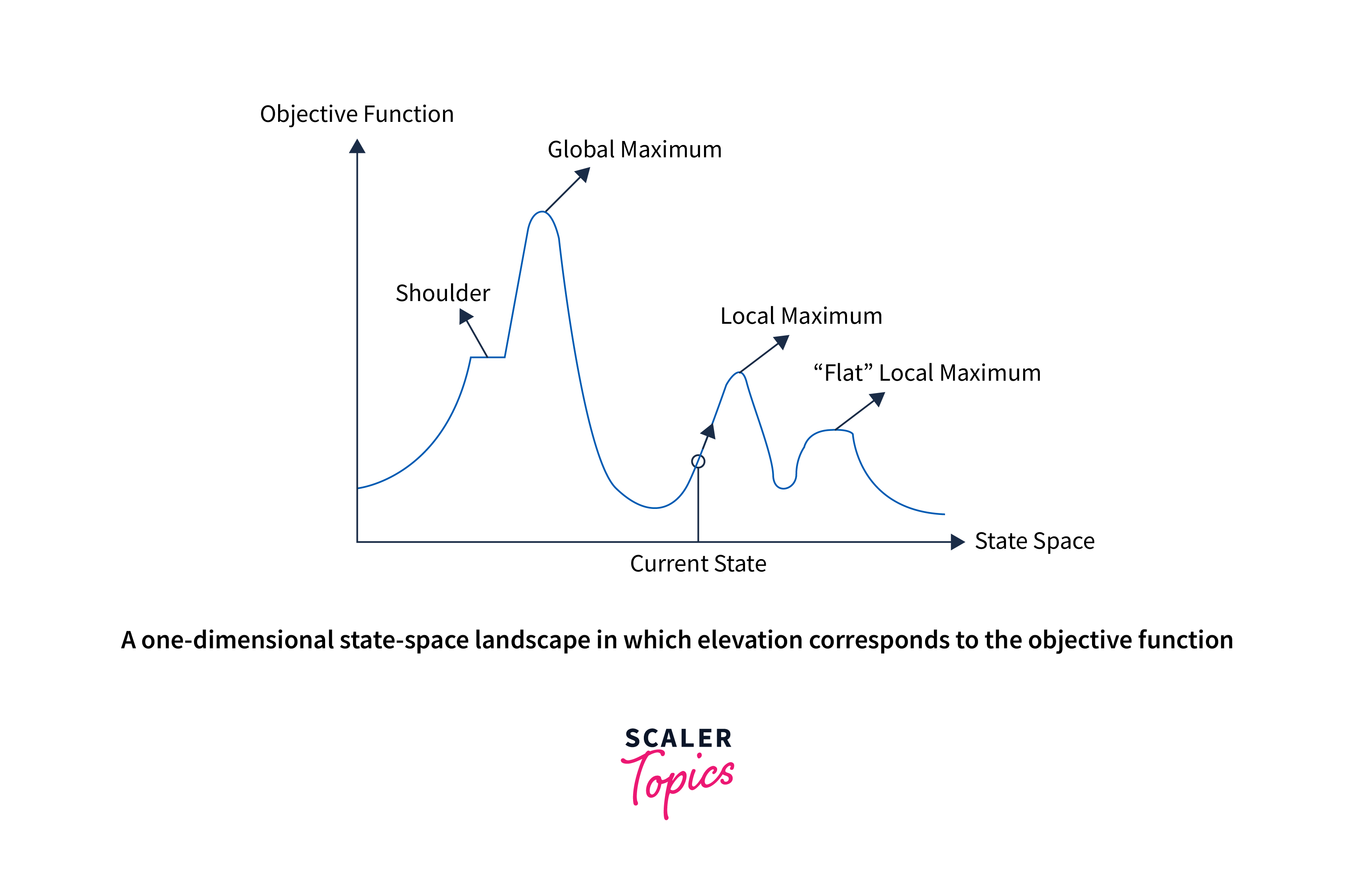
Consider the above figure, representing the goal state/peak and the current state of the climber.

The state-space landscape signifies a graphical representation of the hill-climbing algorithm, which depicts a graph between various states of the algorithm and Objective function/Cost.

The topographical regions shown in the figure can be defined as:

• Global Maximum: It is the highest point on the hill, also the goal state.
• Local Maximum: It is the peak higher than all other peaks but lower than the global maximum.
• Flat local maximum: It is the flat area over the hill with no uphill or downhill. It is a saturated point of the hill.
• Shoulder: It is also a flat area where the summit is possible.
• Current state: It is the person's current position.

On Y-axis, we have taken the objective function or cost function and state space on the x-axis. If the function on Y-axis is cost, then the aim of the search is to find the global minimum and local minimum. If the function of the Y-axis is the cost function, then the goal of the search is to find the local maximum and global maximum.

Algorithm

The algorithm has the following steps:

• Generate an initial solution.
• Evaluate the objective function for the initial solution.
• Generate the neighbours of the current solution.
• Select the neighbour with the highest objective function value.
• If the objective function value of the selected neighbour is better than the current solution, update the current solution with the selected neighbour and repeat step 2.
• Otherwise, terminate the algorithm and return the current solution as the best solution found.

Pseudocode

Types of Hill Climbing Search Algorithm

There are the following types of hill-climbing searches:

• Simple hill climbing
• Steepest-ascent hill climbing
• Stochastic hill climbing
• Random-restart hill climbing

Simple Hill Climbing

Simple hill climbing is the simplest way one can implement a hill-climbing algorithm. It starts with an initial solution and iteratively improves it by making small modifications to the current solution to maximize or minimize an objective function. Finally, the algorithm terminates when no better solution can be found in the immediate neighbourhood of the current solution.

This algorithm has the following features:

• Less time-consuming.
• We get a less optimal solution, and the solution is not guaranteed.

Algorithm

• Generate an initial solution.
• Evaluate the objective function for the initial solution.
• Repeat the following until no better solution can be found:
  • Generate the neighbours of the current solution.
  • Select the neighbor with the highest objective function value.
  • If the objective function value of the selected neighbour is better than the current solution,
  • Update the current solution with the selected neighbour.
  • Update the best solution found so far if the selected neighbour is better than the current best solution.
  • Otherwise, terminate the algorithm and return the current solution as the best solution found.

Steepest-ascent Hill Climbing

The steepest-ascent algorithm is a variation of a simple hill-climbing algorithm. It starts with an initial solution and iteratively improves it by making small modifications to the current solution to maximize or minimize an objective function. However, unlike simple hill climbing, it evaluates all possible neighbours and selects the one with the highest objective function value rather than the first better neighbour.

Algorithm The steps of the steepest-ascent hill climbing algorithm are as follows:

• Initialize the current point to a random starting point.
• Evaluate the value of the function at the current point.
• Generate all neighbouring points of the current point.
• Evaluate the value of the function at each neighbouring point.
• Move to the neighbouring point with the highest (or lowest) function value.
• If the value at the new point is higher (or lower) than the value at the current point, repeat step 3. Otherwise, return the current point as the maximum (or minimum).

Limitation: The limitation of the steepest-ascent hill climbing algorithm is the same as hill climbing, where it can get stuck in a local maximum (or minimum) and fail to find the global maximum (or minimum).

Stochastic Hill Climbing Algorithm

This algorithm starts with an initial solution and iteratively improves the solution by making small random perturbations and accepting the new solution if it is better than the current one. Stochastic hill climbing can effectively find a function's global maximum or minimum when the objective function is noisy, non-convex, or has many local optima.

Algorithm

Here are the main steps of the stochastic hill climbing algorithm:

• Initialize the algorithm by generating an initial solution.
• Evaluate the fitness of the initial solution using the objective function.
• Generate a new solution by making a small random perturbation to the current solution.
• Evaluate the fitness of the new solution using the objective function.
• If the new solution is better than the current one, accept it as the new one.
• If the new solution is worse than the current solution, either reject it or accept it with a certain probability determined by a temperature parameter.
• Repeat steps 3-5 until the stopping criteria are met (e.g., a maximum number of iterations, a minimum improvement threshold, etc.).

Limitation: Like the above algorithms, it can also get stuck in local optima and may only sometimes find the global optimum.

Random-restart Hill Climbing

Random-restart hill climbing is a metaheuristic algorithm used to find a function's global maximum or minimum. The algorithm iteratively applies the hill climbing algorithm from random starting points until a stopping criterion is met. This algorithm can effectively find a function's global maximum or minimum when the objective function has many local optima. Furthermore, by starting from different random points, the algorithm can explore different regions of the search space and increase the likelihood of finding the global optimum.

Algorithm

Here are the main steps of the random-restart hill climbing algorithm:

• Initialize the algorithm by generating a random starting solution.
• Apply the hill climbing algorithm to the starting solution until it reaches a local maximum or minimum.
• If the local maximum or minimum found is better than the best solution, update the best solution.
• Generate a new random starting solution and apply the hill climbing algorithm again.
• Repeat steps 2-4 for a fixed number of iterations or until a stopping criterion is met (e.g., a maximum number of iterations, a minimum improvement threshold, etc.).
• Return the best solution found.

Limitations

Hill climbing algorithms have limitations that can affect their performance in certain situations. Here are some of the main limitations of hill climbing algorithms:

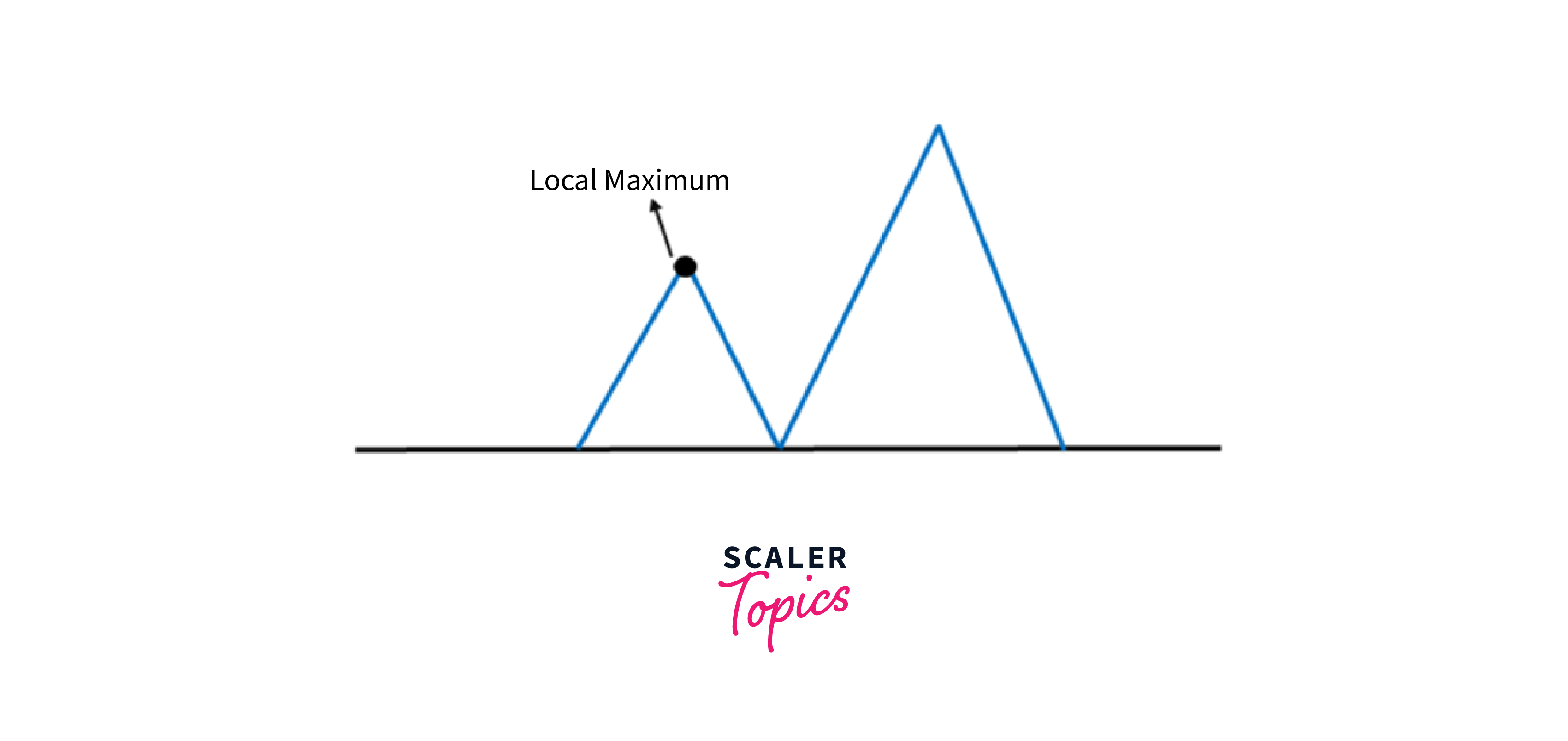
• Local Optima: Hill climbing algorithms can get stuck in local optima and need help finding the global optimum. This occurs when the algorithm converges to a solution that is locally optimal but not globally optimal.

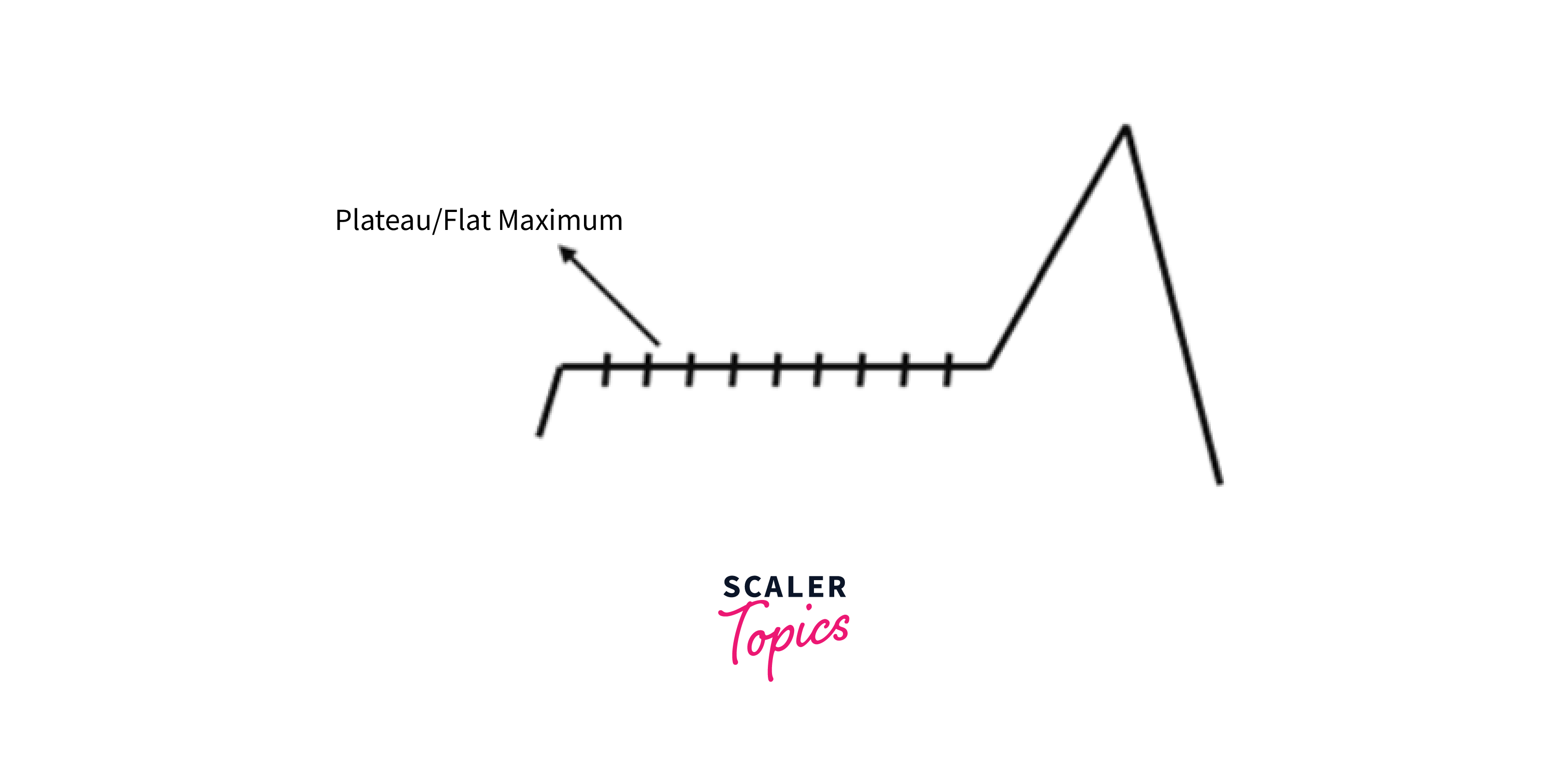
• Plateaus: Plateaus occur when the objective function is flat or nearly flat in certain regions of the search space. In such cases, hill climbing algorithms may take a long to reach the global optimum or get stuck at a local optimum.

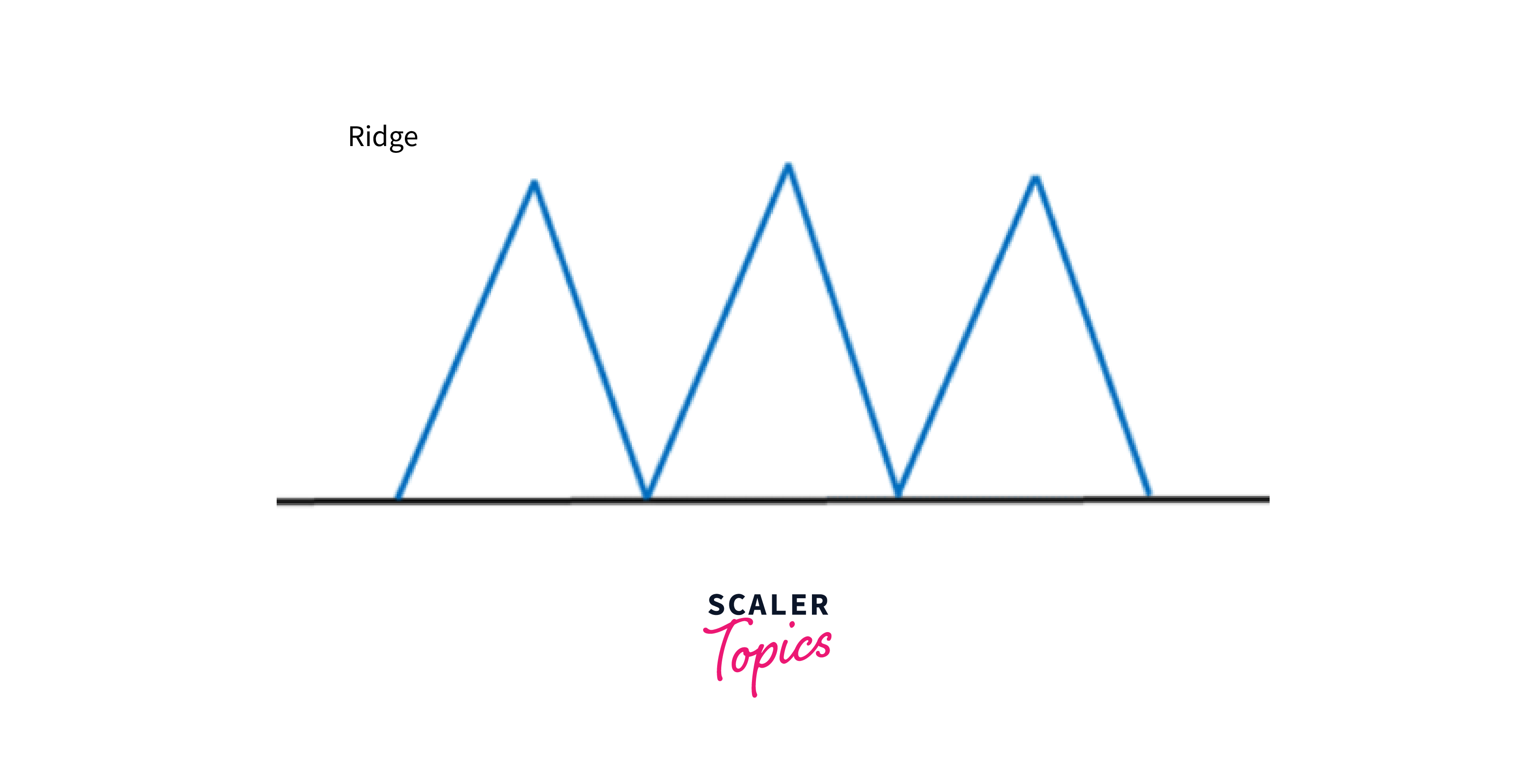
• Ridges: A ridge is a special form of the local maximum, which has a higher area than its surrounding but itself has a slope that cannot be reached in a single move.

• Multiple Solutions: In some cases, there may be multiple global optima or nearly optimal solutions. Hill climbing algorithms may only be able to find some of these solutions.

• Initial Solution Dependency: Hill climbing algorithms are sensitive to the initial solution. Therefore, depending on the starting point, the algorithm may converge to different local optima.

• Limited Search: Hill climbing algorithms explore the search space locally and may not consider global information about the objective function.

• Efficiency: Hill climbing algorithms can be computationally expensive if the search space is large or complex.

Various modifications and extensions to the hill climbing algorithm have been proposed to overcome these limitations, such as simulated annealing, genetic algorithms, and tabu search.

Local Beam Search

Local beam search is a heuristic search algorithm used to solve optimization problems by exploring the search space. This algorithm explores a graph by expanding the most optimistic node in a limited set.

Beam search uses breadth-first search(bfs) to build its search tree. At each level of the tree, it works by generating all successors of the states at the current level. It then sorts them in increasing order of heuristic cost. Most importantly, it stores a predetermined number (β) of best states at each level. We call this the beamwidth. Only those states are expanded next. The beamwidth bounds the memory required to perform the search.

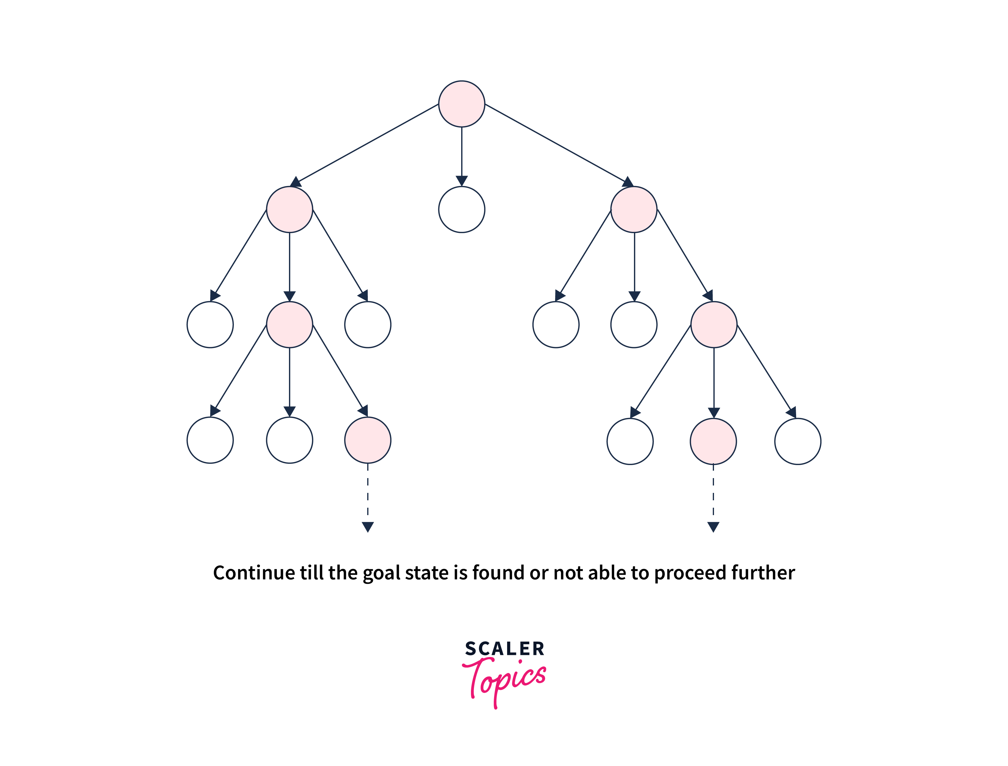
Algorithm

• Initialize the algorithm by generating k random starting solutions.
• Evaluate the fitness of each starting solution using the objective function.
• Choose the top m solutions (where m < k) as the new starting solutions for the next iteration. This is called the beam width.
• Generate new candidate solutions by making small random perturbations to the current solutions.
• Evaluate the fitness of each new solution using the objective function.
• Choose the top m solutions as the new solutions for the next iteration.
• Repeat steps 4-6 until a stopping criterion is met (e.g., a maximum number of iterations, a minimum improvement threshold, etc.).
• Return the best solution found.

Local beam search maintains a set of k candidate solutions at each iteration and selects the top m solutions as starting solutions for the next iteration. This approach allows the algorithm to explore different regions of the search space and converge to better solutions.

Limitation: One limitation of local beam search is that it can get stuck in local optima. To overcome this, algorithm variants have been proposed, such as stochastic local beam search and beam search with random restarts.

Simulated Annealing

Simulated Annealing is a probabilistic optimization algorithm used to find the global minimum of a function by iteratively adjusting a candidate solution to the function. The annealing process inspired the algorithm in metallurgy, which is the process of heating a material until it reaches an annealing temperature. Then it will be cooled down slowly to change the material to the desired structure.

The basic idea of simulated annealing is to start with an initial solution and then randomly change it to produce a new solution.

The change can improve or worsen the solution, depending on the optimized function. The algorithm then evaluates the new solution and decides whether to accept or reject it based on a probability function that depends on the current temperature and the degree of worsening in the solution.

As the algorithm progresses, the temperature gradually lowers, reducing the probability of accepting worse solutions. This process allows the algorithm to escape local minima and converge towards the global minimum of the function.

Simulated annealing has been applied to many optimization problems, including combinatorial optimization, machine learning, and physics. It is particularly useful in cases where the optimized function is highly complex or has many local minima such that algorithms like Gradient Descent would be stuck at.

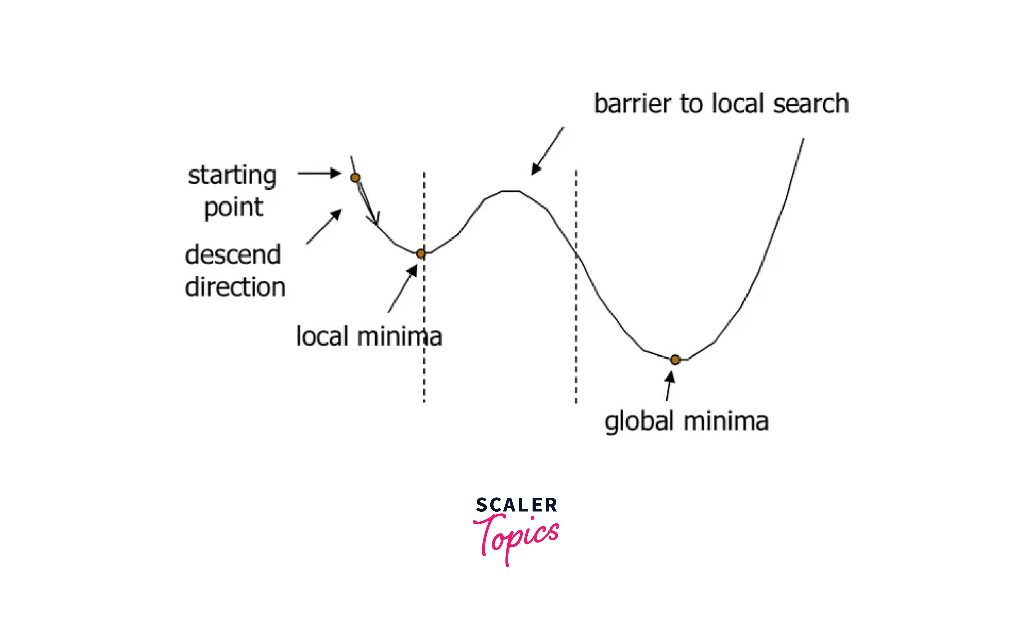
In problems like the one above, if Gradient Descent started at the starting point indicated, it would be stuck at the local minima and unable to reach the global minima.

However, the algorithm can be computationally expensive, especially for large search spaces, and requires careful tuning of the cooling schedule and probability function.

Algorithm

The Simulated Annealing algorithm can be summarized in the following steps:

• Initialize a candidate solution. This could be a random solution or a known starting point.

• Define an objective function that measures the quality of a solution. This function should return a numerical value reflecting the solution's quality.

• Set the initial temperature, cooling rate, and stopping criterion.

• Repeat the following steps until the stopping criterion is met:

  a. Generate a new candidate solution by randomly modifying the current solution.

  b. Evaluate the objective function for the new candidate solution.

  c. Calculate the change in objective function value between the current and new candidate solutions.

  d. If the new solution is better than the current solution, accept the new solution as the current solution.

  e. If the new solution is worse than the current solution, calculate the probability of accepting the new solution based on the current temperature and the degree of worsening. Accept the new solution if the probability is greater than a random number between 0 and 1. Otherwise, reject the new solution and keep the current solution.

  f. Lower the temperature according to the cooling rate.

• Return the best solution found during the algorithm.

The acceptance probability function can be defined in different ways, but a common choice is the Boltzmann distribution:

Where $\Delta E$ is the change in objective function value between the current and new candidate solutions, $T$ is the current temperature, and $e$ is the base of the natural logarithm. The probability function decreases as the temperature decreases and the degree of worsening increases, making it less likely to accept worse solutions as the algorithm progresses.

What are Genetic Algorithms?

A genetic algorithm is a search heuristic inspired by Charles Darwin's theory of natural evolution. They are a class of optimization algorithms inspired by natural selection and genetics principles. They are used to solve problems in various domains, including engineering, economics, and artificial intelligence.

This algorithm reflects the process of natural selection, where the fittest individuals are selected for reproduction to produce offspring of the next generation.

The basic idea behind genetic algorithms is to generate a population of candidate solutions to a problem and then use evolutionary operators such as mutation, crossover, and selection to create new generations of solutions. The process continues until a satisfactory solution is found.

The Notion of Natural Selection

The process of natural selection produces offspring that inherit the parents' characteristics and will be added to the next generation. It starts with the selection of the fittest individuals from a population.

If parents have better fitness, their offspring will be better than parents and have a better chance of surviving. This process keeps on iterating, and in the end, a generation with the fittest individuals will be found.

Algorithm

The genetic algorithm process can be summarized in the following steps:

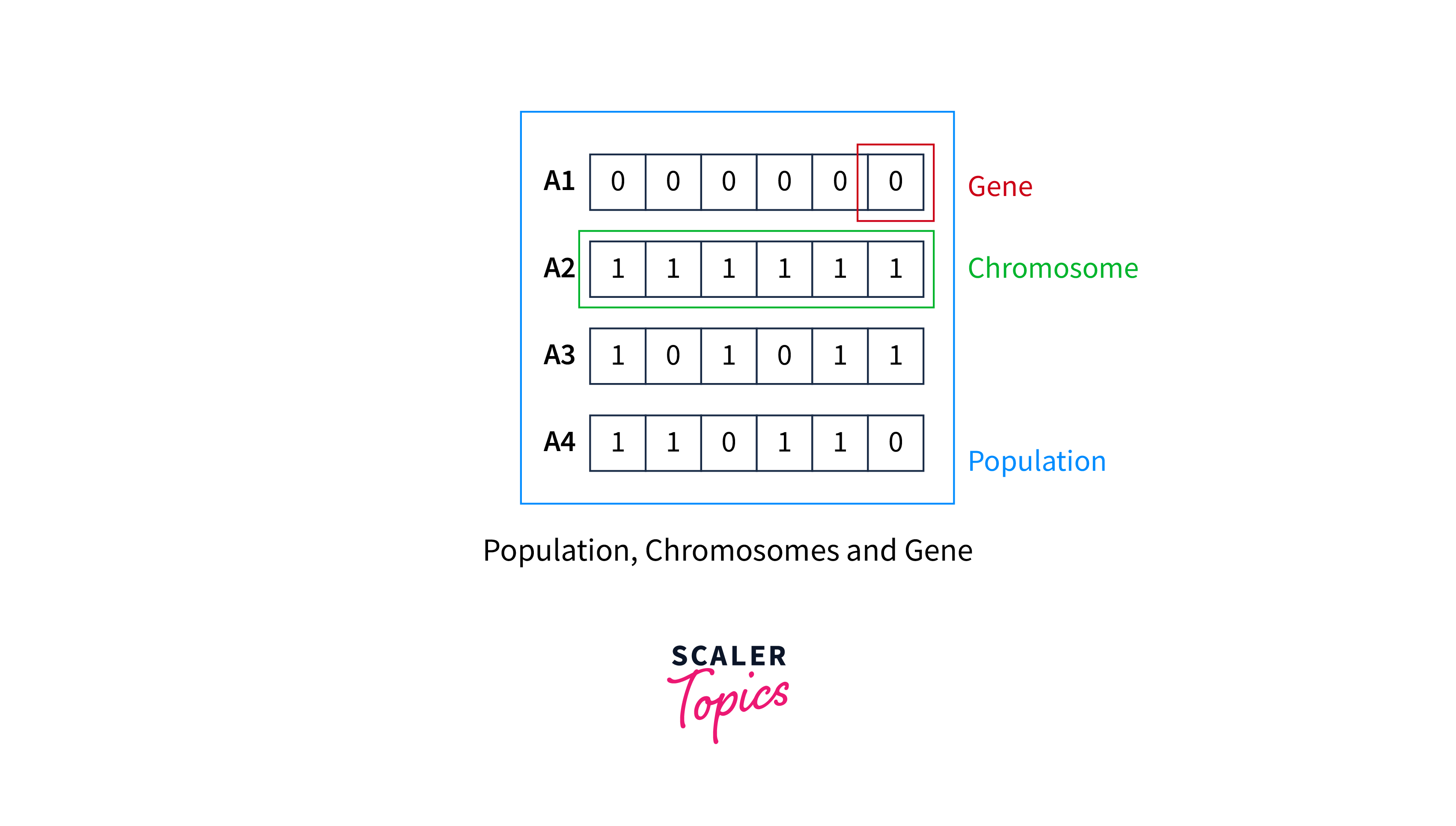
• Initialization or initial population: The process begins with a set of individuals called a Population. Each individual is a solution to the problem you want to solve. A population of potential solutions is randomly generated.

An individual is characterized by a set of parameters (variables) known as Genes. Genes are joined into a string to form a Chromosome (solution).

• Evaluation(Fitness function): Each solution in the population is evaluated and assigned a fitness score based on how well it solves the problem. The fitness function determines how to fit an individual (an individual's ability to compete with others).

• Selection: Solutions with higher fitness scores are more likely to be selected for the next generation. Various methods, including tournament selection, roulette wheel selection, and rank-based selection, do this.

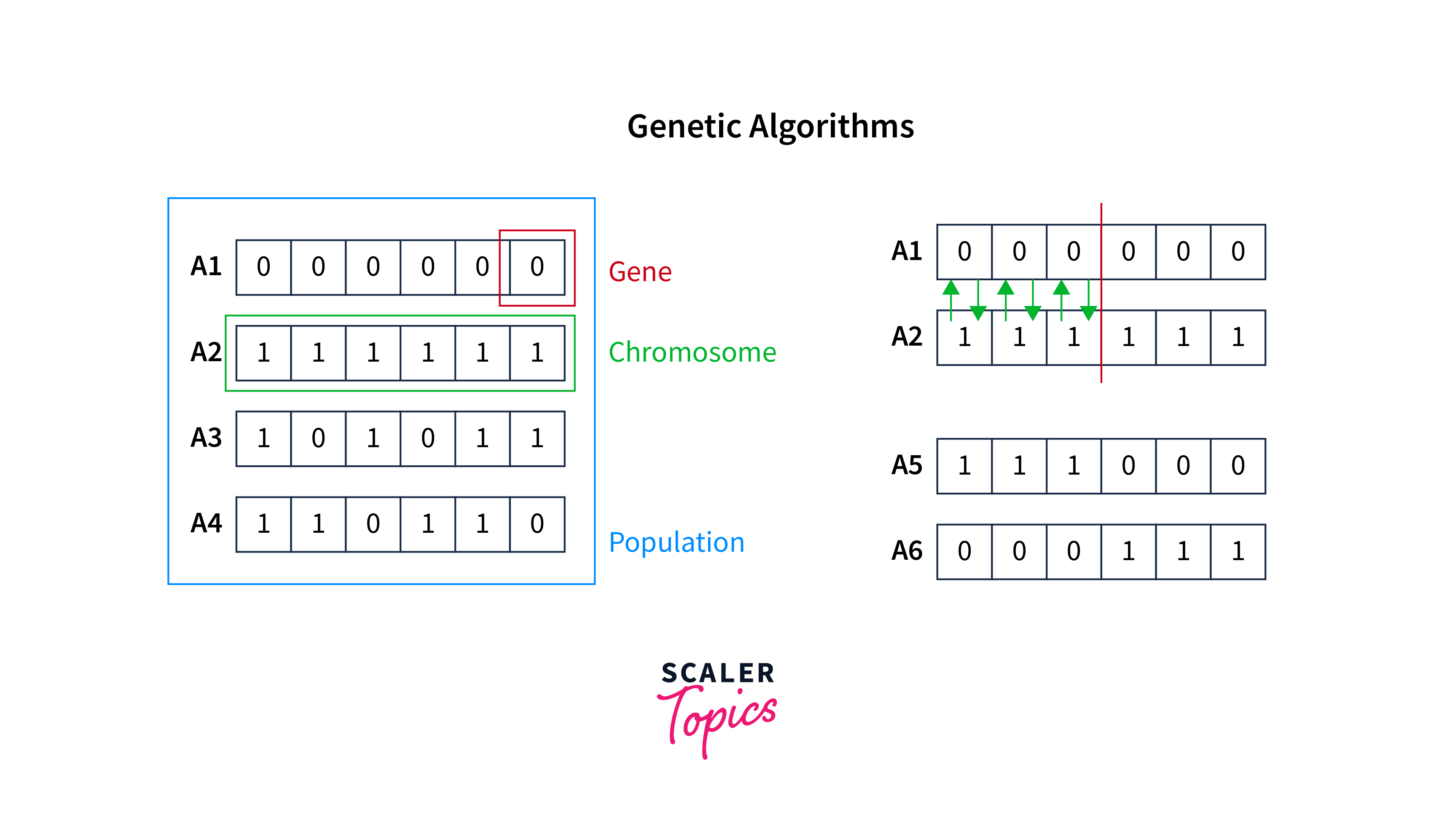
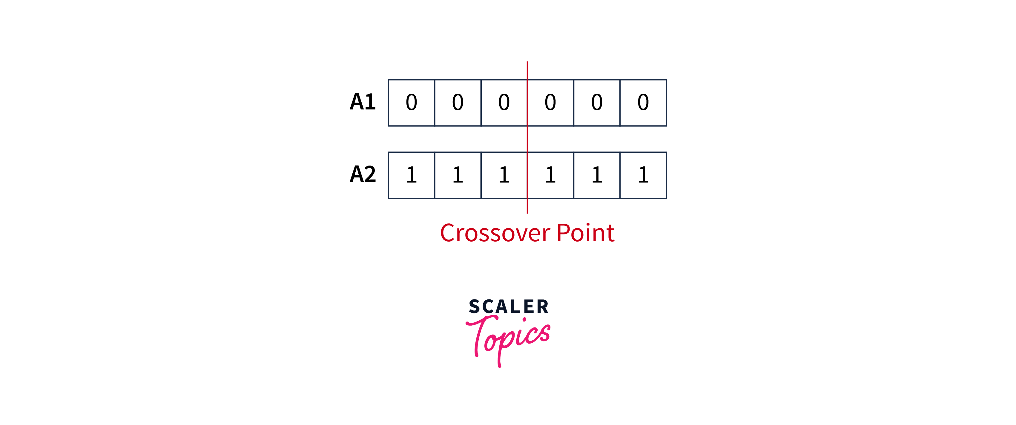
• Crossover: Selected solutions are combined through crossover, which creates a new set of solutions by swapping or mixing parts of the selected solutions.

A crossover point is chosen randomly from within the genes for each pair of parents to be mated. For example: A crossover point as three would look like:-

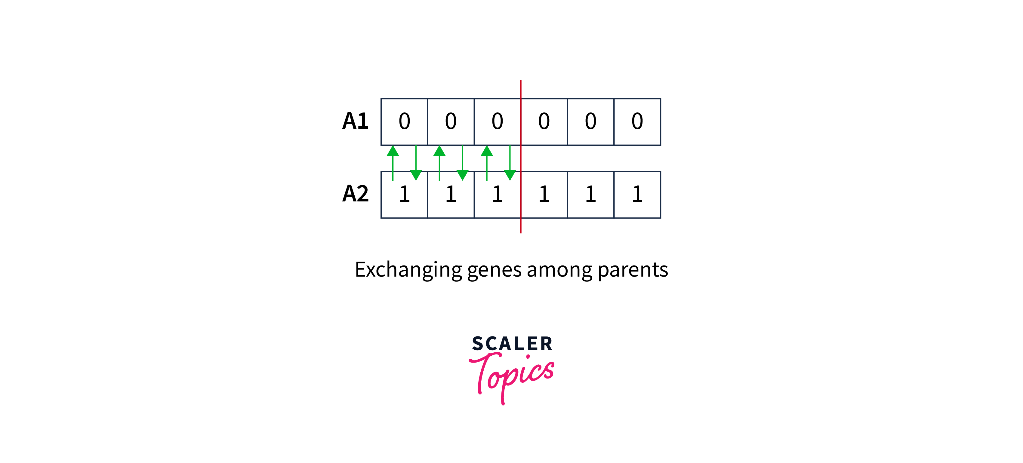
Offspring are then generated by exchanging the parents' genes until the crossover point is reached.

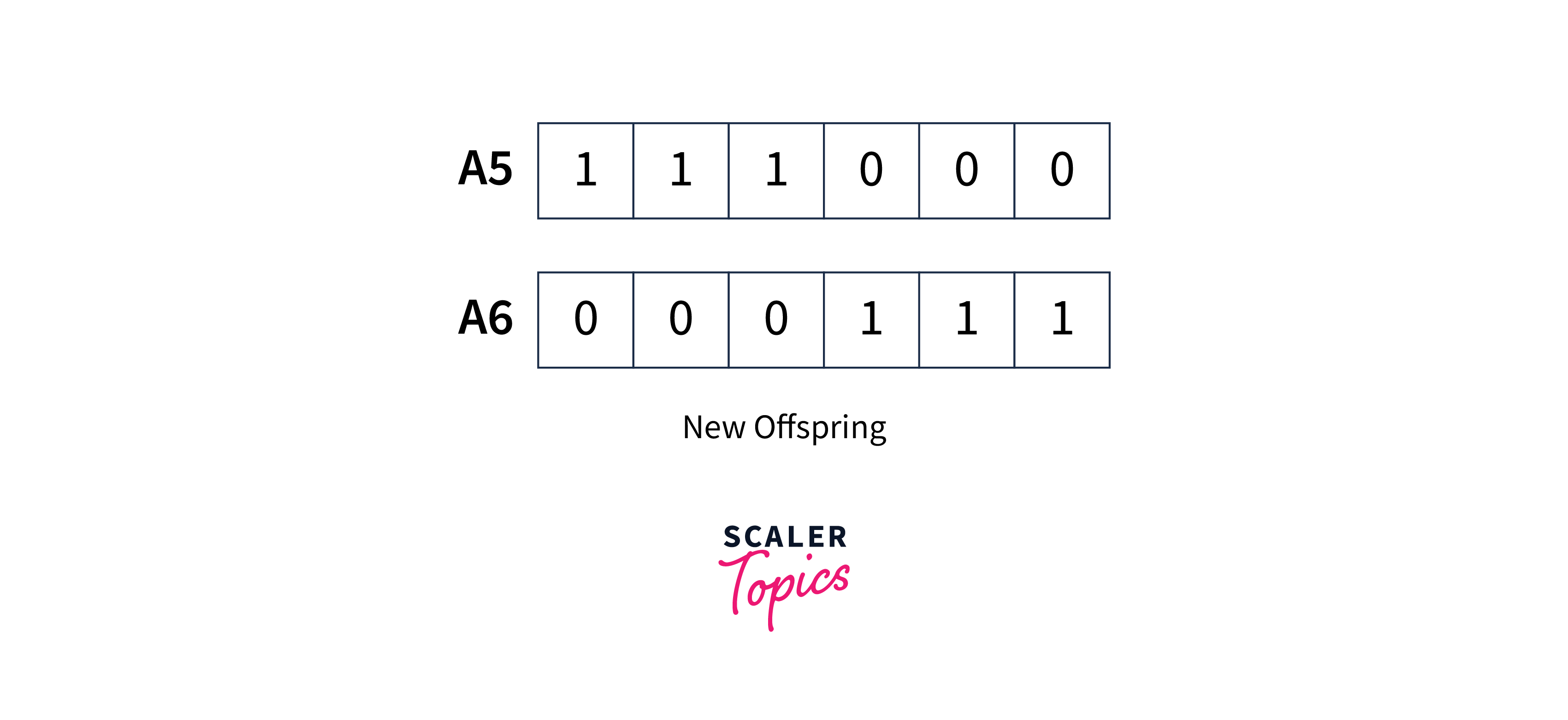
The new offsprings obtained are:-

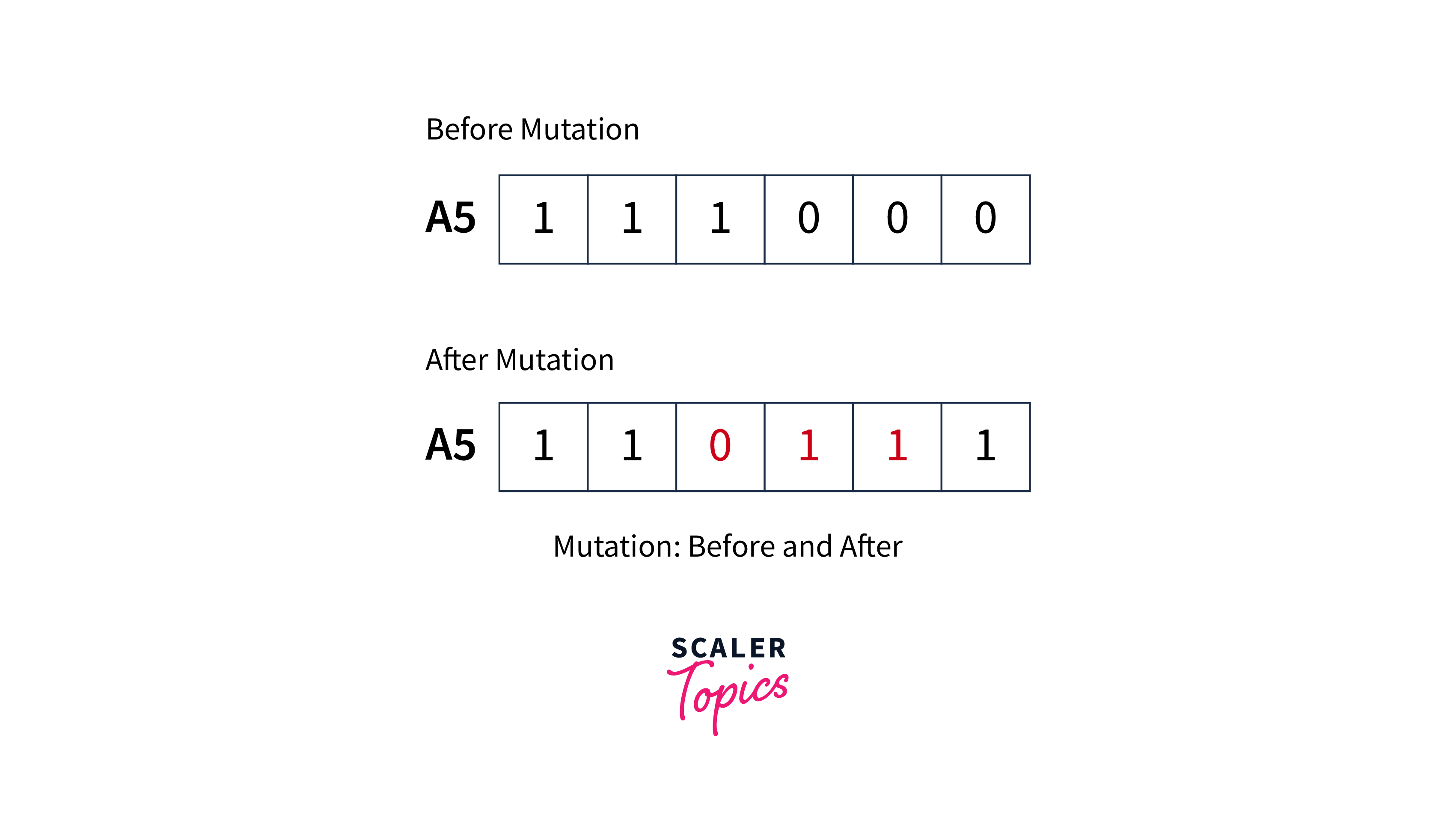
• Mutation: Some newly created solutions undergo mutation, which randomly changes some of their characteristics.This implies that some bits in the bit string can be flipped.

• Replacement: The new generation of solutions replaces the previous generation, and the process repeats from step 2 until a satisfactory solution is found.

Genetic algorithms have advantages over other optimization methods, such as searching large solution spaces and handling multiple objectives.

However, they can be computationally expensive and require careful tuning of the parameters.

They are often used with other techniques, such as local search or simulated annealing, to improve performance.

What is the Travelling Salesman Problem?

The Travelling Salesman Problem (TSP) is a well-known optimization problem in artificial intelligence. The problem involves finding the shortest possible route a salesman can take to visit a set of cities and return to the starting city, visiting each city exactly once.

In more formal terms, the TSP can be defined as given a set of n cities and a distance matrix d that specifies the distance between each pair of cities. The goal is to find a permutation of the cities (i.e., a specific order to visit the cities) that minimizes the total distance traveled.

The problem is known to be NP-hard, meaning that no known efficient algorithm can solve it exactly for all instances.

Many algorithms have been developed to solve the Travelling Salesman Problem (TSP), including exact algorithms, heuristics, and metaheuristics. Here are some of the popular ones:

• Brute Force Algorithm: This algorithm generates all possible city permutations and calculates the total distance travelled for each permutation. The solution with the shortest distance is selected as the optimal solution. However, this algorithm is only practical for small problem sizes as the number of permutations increases exponentially with the number of cities.

• Nearest Neighbor Algorithm: This algorithm starts at a random city and repeatedly selects the nearest unvisited city until all cities have been visited. The resulting tour is not guaranteed optimal but is usually reasonably good for large instances of the problem.

• Genetic Algorithm: This algorithm is a metaheuristic that uses principles of natural selection and evolution to improve a population of candidate solutions iteratively. The algorithm starts with a randomly generated population of tours and iteratively selects the best individuals to create the next generation of solutions.

• Simulated Annealing: This algorithm is another metaheuristic that uses a probabilistic approach to search for the optimal solution. The algorithm starts with an initial solution and then iteratively perturbs the solution and accepts or rejects the new solution based on a probability distribution.

• Ant Colony Optimization: This algorithm is inspired by the behavior of ants and their pheromone trails. The algorithm uses a population of artificial ants to iteratively construct candidate solutions by selecting the next city to visit based on the amount of pheromone present on the path between cities.

Many other algorithms have been developed to solve the TSP, and the choice of algorithm depends on the specific problem instance and the desired trade-off between solution quality and computational efficiency.

Limitations of Local Search Algorithms

• Local Optima: Local search algorithms can get stuck in local optima, where the current solution is the best in its immediate neighborhood but not globally optimal. Once trapped in a local optimum, the algorithm can only find better solutions by making larger-scale changes that may be computationally expensive.

• Sensitivity to Initial Solution: Local search algorithms are often sensitive to the initial solution used as a starting point. A poor initial solution can result in the algorithm converging to a suboptimal solution, while a good initial solution can lead to finding the global optimum.

• Lack of Diversity: Local search algorithms can converge to a limited set of solutions that are very similar to each other and may not explore a wide range of potential solutions.

• Limited Scope of Search: Local search algorithms are often limited to exploring only a small subset of the solution space and may miss potentially better solutions outside the explored region.