Excel AVERAGEIF Function
Overview
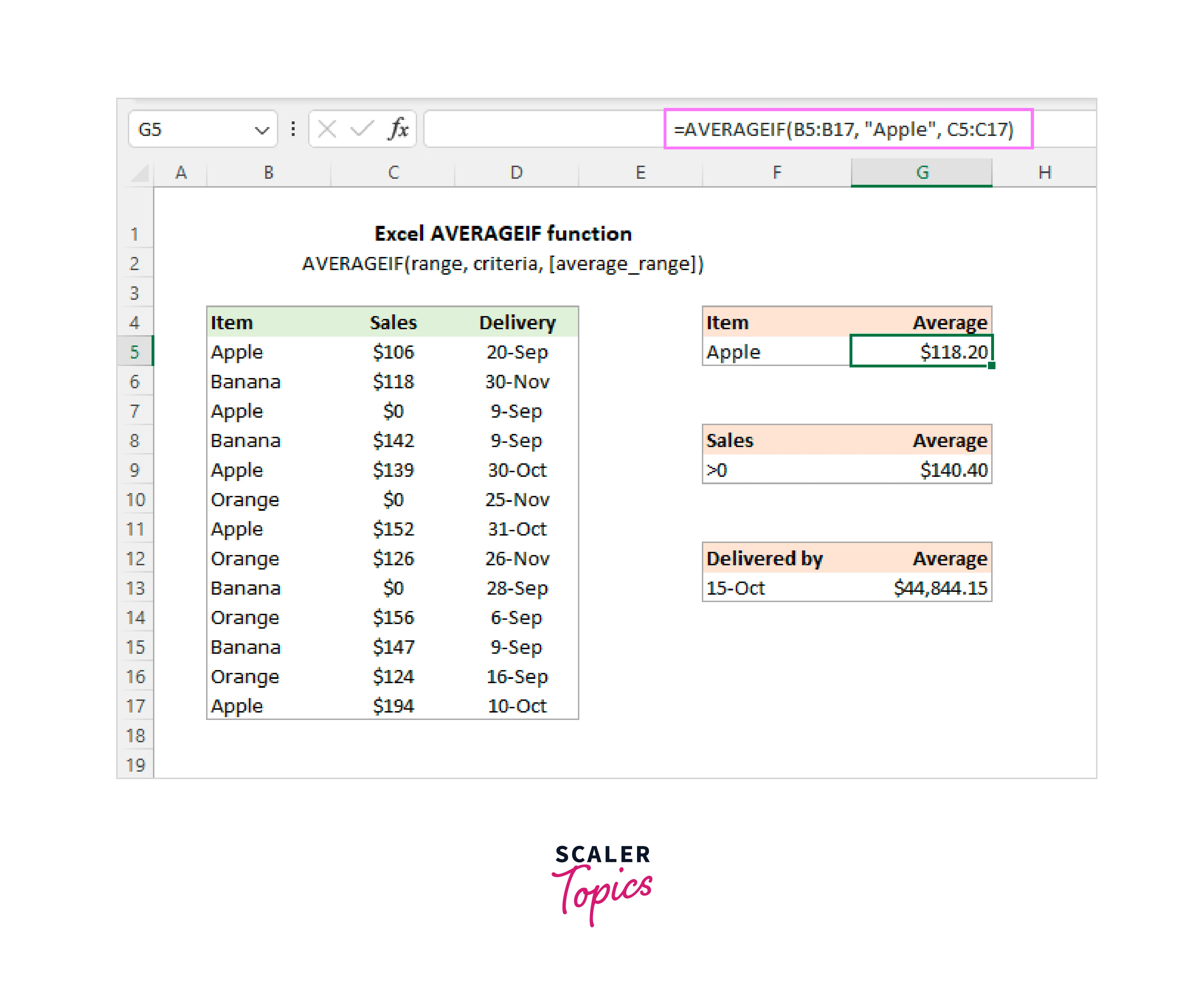
Excel's AVERAGEIF function is a powerful tool for calculating the average of a range of values based on a specified condition or criteria. It allows users to filter data and compute the average of only those values that meet the defined criteria.
AVERAGEIF takes three main arguments: the range of cells to evaluate, the criteria to apply, and the range of values to average. You can use various comparison operators (like greater than, less than, equal to) and wildcards to define your criteria, making it flexible for different scenarios. This function is invaluable for analyzing data sets where you need to find the average of specific subsets, such as sales data for a particular product, employee performance ratings above a certain threshold, or any other customized calculations. Excel's AVERAGEIF function simplifies data analysis and aids in informed decision-making.
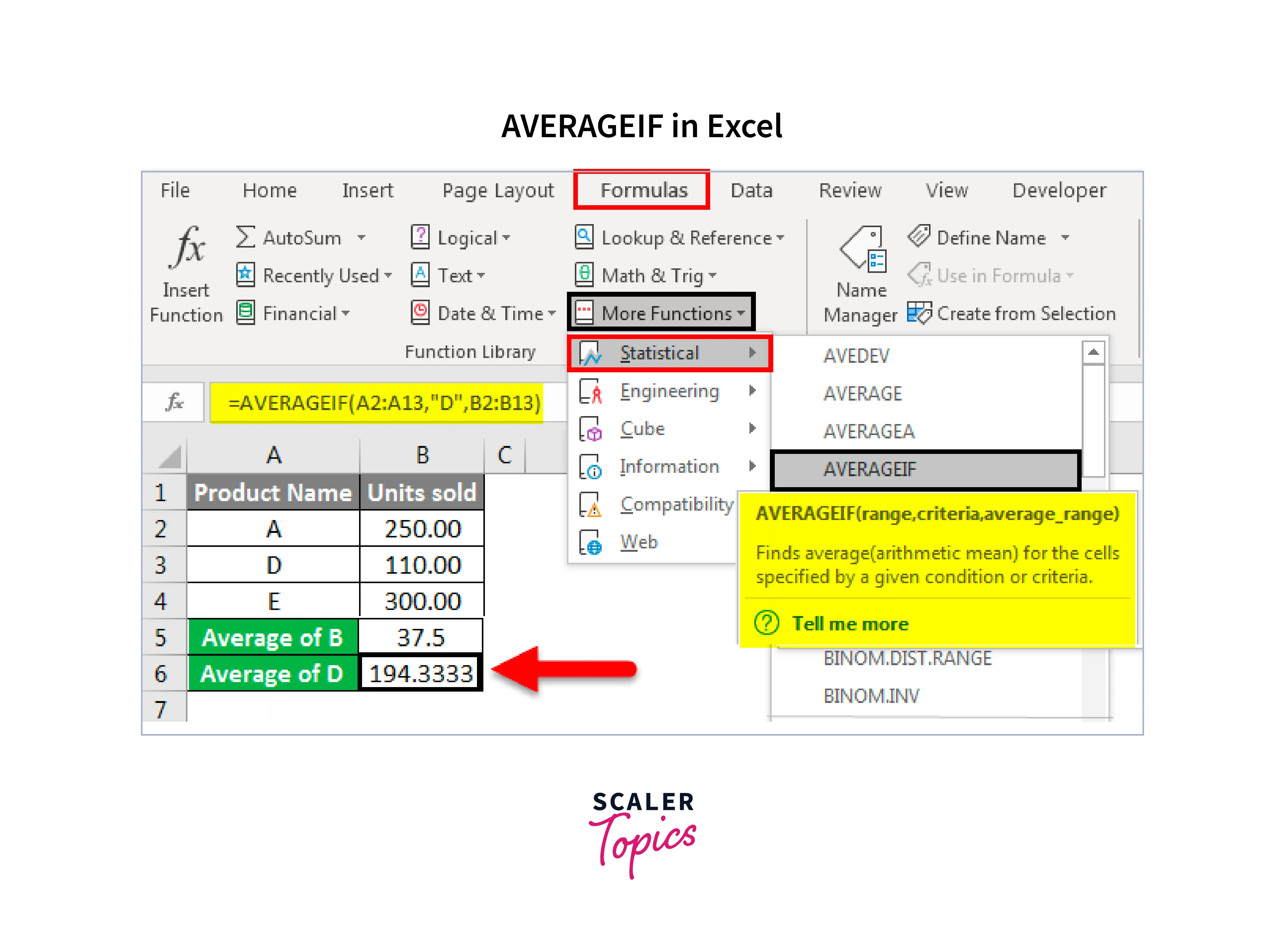
Syntax of AVERAGEIF Function in Excel
The AVERAGEIF function in Excel calculates the average of a range of numbers based on a given condition or criteria. Its syntax consists of three main arguments, and you can use additional optional arguments in certain cases.
Here's the detailed syntax of the AVERAGEIF function:
Parameters of Excel AVERAGEIF Function
- Range (required): This is the range of cells that you want to evaluate against a specified condition or criteria. It represents the set of values from which you want to calculate the average.
- Criteria (required): This is the condition or criteria that you want to apply to the values in the range. You specify what values to include in the average based on this condition. It can be a number, expression, or text enclosed in double quotes. You can use various comparison operators and wildcards, such as:
- Greater than: >
- Less than: <
- Greater than or equal to: >=
- Less than or equal to: <=
- Equal to: =
- Not equal to: <>
- Wildcards like * (matches any sequence of characters) and ? (matches any single character) when dealing with text.
- average_range (optional): This parameter specifies the range of cells that you want to calculate the average for. It is used when you want to average a different range of cells than the one specified in the range parameter. If this argument is omitted, Excel uses the same range for both evaluating the criteria and calculating the average.
Return Value of Excel AVERAGEIF Function
- Function Purpose: AVERAGEIF is used to calculate the average of values that meet a certain condition. It's particularly useful when you have a range of data, and you want to find the average of a specific subset of values that satisfy a particular criterion.
- Parameters:
- Range (required): This is the range of cells you want to evaluate.
- Criteria (required): This is the condition or criteria you want to apply to the values in the range.
- average_range (optional): This is the range of cells that contains the values you want to average. If omitted, Excel uses the same range for both evaluating the criteria and calculating the average.
- Calculation:
- Excel evaluates each value in the specified range against the given criteria. It includes only the values that meet the condition in the calculation.
- If you've specified an average_range, Excel calculates the average of the values in that range that correspond to the values meeting the criteria in the range.
- If you haven't specified an average_range, Excel calculates the average of the values in the range that meet the criteria.
- Return Value: The AVERAGEIF function returns a single numeric value, which is the calculated average of the values that meet the specified condition.
Examples of Excel AVERAGEIF Function
Basic Example
Suppose you have a list of test scores in cells A1 to A10, and you want to calculate the average of scores that are greater than or equal to 80.
Here's how you can use the AVERAGEIF function to do this:
- In an empty cell, type the following formula:
Press Enter. The function will calculate the average of the scores in the range A1:A10 that meet the condition greater than or equal to 80.
Assuming your scores are as follows:
- A1: 85
- A2: 90
- A3: 78
- A4: 92
- A5: 76
- A6: 88
- A7: 95
- A8: 82
- A9: 79
- A10: 87
The AVERAGEIF function will include the scores 85, 90, 92, 88, 95, 82, and 87 because they are greater than or equal to 80, and it will calculate their average.
Double Quotes ("") in Criteria
Here's how you can use double quotes within the criteria parameter of AVERAGEIF:
Suppose you have a list of products in cells A1 to A10, and you want to calculate the average price for a specific product, like "Apples." You would use double quotes to specify the criteria:
In this example:
- A1:A10 represents the range of products.
- "Apples" is the criteria enclosed in double quotes. This specifies that you want to calculate the average for the product named "Apples."
- B1:B10 represents the range of prices corresponding to the products.
- The AVERAGEIF function will only include prices where the product name matches "Apples" based on the criteria in double quotes. It will then calculate the average of those prices.
So, in this case, the formula will calculate the average price for "Apples" in your dataset.
Wildcards
Wildcards in Excel's AVERAGEIF function are often used when you have criteria involving partial text matching or patterns. The two main wildcards used are the asterisk (*) and question mark (?).
Let's say you have a list of products in cells A1 to A10 and you want to calculate the average price for products that contain the word "Apple" anywhere in their names, regardless of what comes before or after "Apple." You can use a wildcard asterisk (*) to achieve this:
- A1:A10 represents the range of products.
- "Apple" is the criteria with wildcards. The asterisk (*) before and after "Apple" means it will match any product name containing "Apple," such as "Apple Pie," "Green Apples," or "Red Apple Juice."
- B1:B10 represents the range of prices corresponding to the products.
- The AVERAGEIF function will calculate the average price for all products that contain "Apple" in their names, regardless of what other text is in the product names.
Average Numbers Ignore Zero
Suppose you have a range of numbers in cells A1 to A5, and you want to calculate the average of these numbers while ignoring any zeroes in the calculation. You can use the AVERAGEIF function as follows:
This formula calculates the average of the numbers in cells A1 to A5, excluding any cells with the value of zero.
Value From Another Cell:
Let's say you have a number in cell B1, and you want to calculate the average of a range of numbers in cells A1 to A5, but you want to use the value in cell B1 as the criterion for averaging. You can use the AVERAGEIF function like this:
This formula calculates the average of the numbers in cells A1 to A5 that match the value in cell B1.
Average and Ignore Errors:
If you have a range of numbers in cells A1 to A5, and some cells contain errors (like #DIV/0! or #N/A), you can calculate the average of the valid numbers while ignoring the errors. You can use the AVERAGEIF function with the criteria to exclude errors:
Conclusion
- Flexible Criteria: AVERAGEIF is a powerful Excel function that calculates the average of a range of values based on a specified condition or criteria.
- Simple Syntax: Its syntax is straightforward, with just three main parameters: range, criteria, and an optional average_range. This simplicity makes it user-friendly even for Excel beginners.
- Text and Numeric Criteria: You can use AVERAGEIF with both text and numeric criteria. It's versatile enough to handle various data types and conditions.
- Wildcards: AVERAGEIF supports wildcards like * and ? for pattern matching, allowing you to find averages based on partial text matches or patterns.