Conditional Formatting in Excel

Conditional Formatting Example

Suppose you have a sales data spreadsheet with a list of products in column A and their corresponding sales figures in column B. You want to highlight the top-selling products based on their sales values.

• Select the range of cells containing the sales figures (column B in this case).
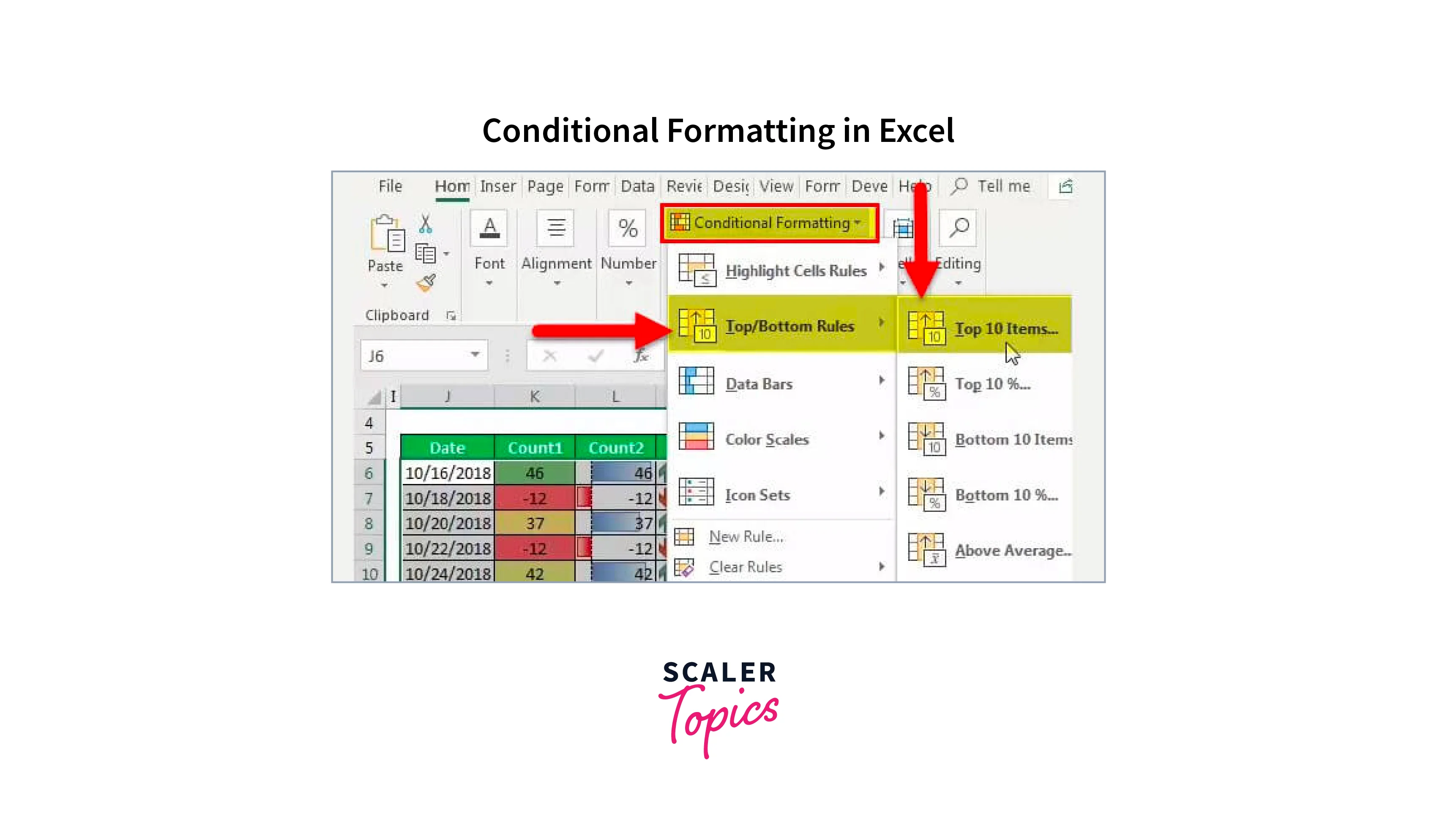
• From the Excel ribbon, navigate to the "Home" tab and click on the "Conditional Formatting" dropdown menu.
• Choose "Top/Bottom Rules" and then select "Top 10 Items" from the submenu. Alternatively, you can choose "New Rule" to create a custom formatting rule.
• In the "Top 10 Items" dialog box, specify the number of top items you want to highlight. For this example, let's choose "10".
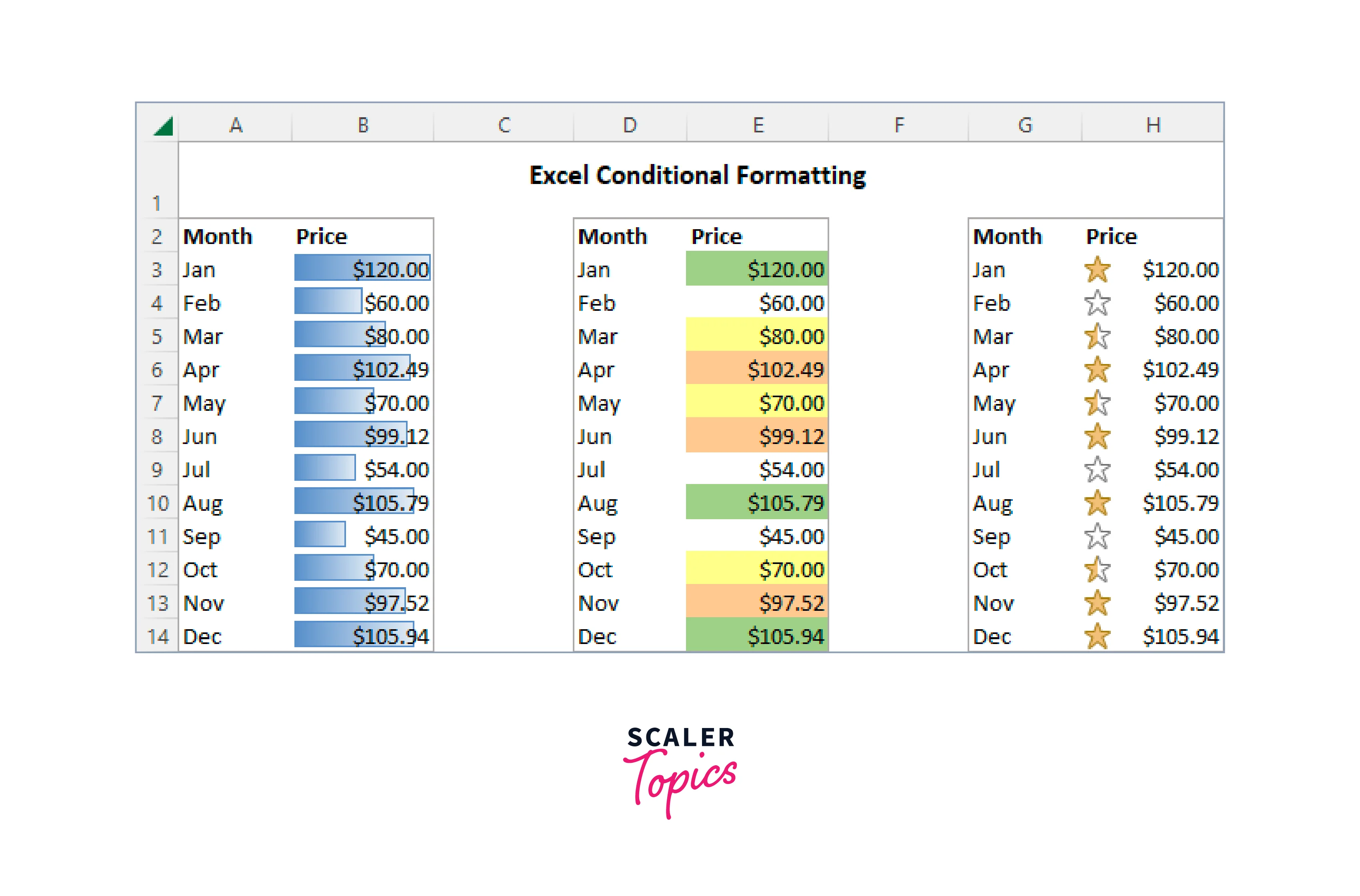
• Select the formatting style you prefer from the available options, such as color scales, data bars, or icon sets. You can customize the formatting style further if needed.
• Click "OK" to apply the Conditional Formatting.

Now, the top 10 sales figures in column B will be automatically highlighted according to the chosen formatting style. The highest value will receive the strongest formatting, gradually decreasing for the subsequent values.

This example demonstrates how Conditional Formatting can be used to quickly identify the top-selling products in a sales dataset. The highlighted cells make it easy to identify the most significant data points at a glance, aiding in data analysis and decision-making.

Color Scale Formatting Example

Suppose you have a spreadsheet containing a list of students in column A and their corresponding test scores in column B. You want to apply Color Scale Formatting to highlight the performance of students based on their test scores.

• Select the range of cells containing the test scores (column B in this case).
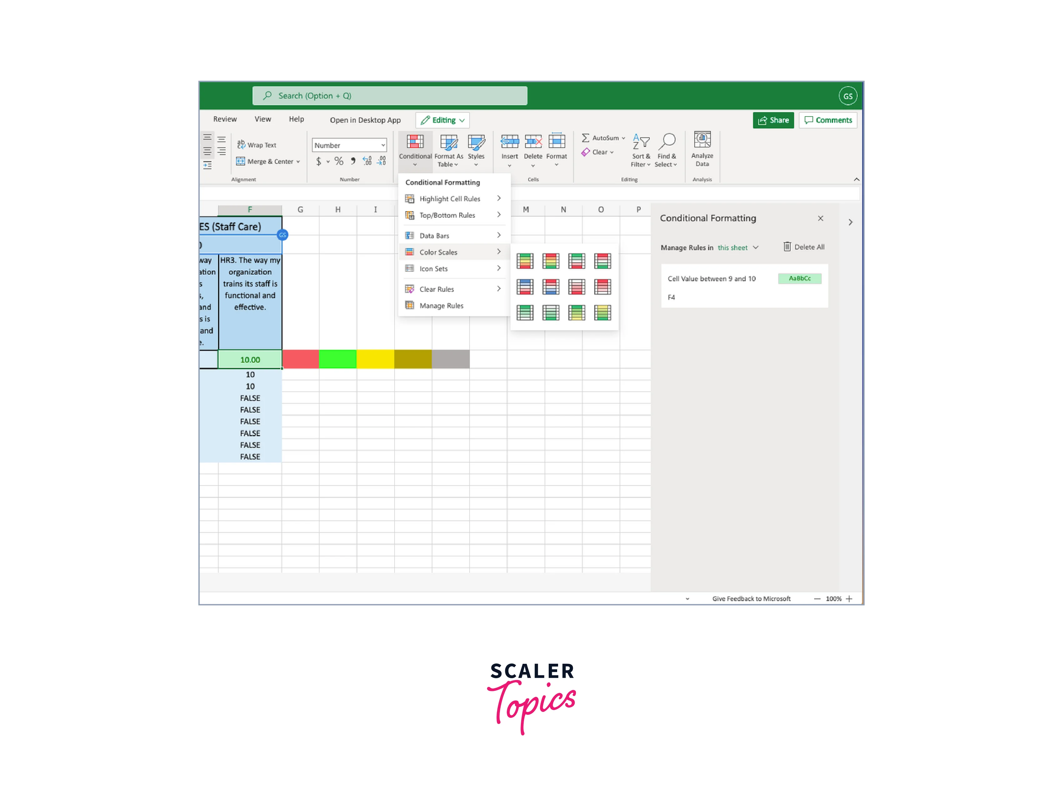
• Go to the "Home" tab in the Excel ribbon and click on the "Conditional Formatting" dropdown menu.
• Select "Color Scales" from the options, and then choose the desired color scale option from the available presets. For example, you can choose the "Red-Yellow-Green Color Scale" to indicate low, medium, and high scores respectively.
• Excel will automatically apply the color scale to the selected range based on the values present. The lowest value will be assigned the color from the lowest end of the scale (red), while the highest value will be assigned the color from the highest end (green). Intermediate values will be assigned colors based on their position within the range.
• Now, the test scores will be visually represented with different colors, making it easier to identify performance levels. Students with low scores will be highlighted in red, those with moderate scores in yellow, and those with high scores in green.

How to Use Conditional Formatting in Excel

Conditional formatting in Excel allows you to format cells based on specific conditions or rules. It helps you highlight important information, identify trends, and visualize data in a meaningful way. Here's a step-by-step guide on how to use conditional formatting in Excel:

• Step 1: Select the cells or range of cells that you want to apply conditional formatting to. You can click and drag to select multiple cells or use Ctrl+Click to select non-contiguous cells.
• Step 2: Go to the "Home" tab in the Excel ribbon.
• Step 3: In the "Styles" group, click on the "Conditional Formatting" button. A dropdown menu will appear with various options.
• Step 4: Choose one of the available options for conditional formatting. For example, you can select "Highlight Cells Rules" to apply formatting based on cell values, or "Top/Bottom Rules" to format the top or bottom values in a range.
• Step 5: Once you've selected an option, another submenu will appear with different formatting rules. Choose the rule that best fits your needs. For instance, if you selected "Highlight Cells Rules," you can choose "Greater Than" to format cells that are greater than a specified value.
• Step 6: After selecting a rule, a dialog box will open where you can specify the formatting details. Enter the criteria or values you want to use for formatting, such as a specific number, text, or a formula. You can also choose the formatting style, such as font color, fill color, or cell borders.
• Step 7: Click "OK" to apply the conditional formatting to the selected cells. Excel will automatically format the cells that meet the specified criteria.
• Step 8: If you want to modify or remove the conditional formatting, select the cells with the formatting and go back to the "Conditional Formatting" button in the "Home" tab. From the dropdown menu, you can choose options like "Manage Rules" to edit or delete existing rules.

Create a New Conditional Formatting Rule

To create a new conditional formatting in Excel, follow these steps:

• Step 1: Select the cells or range of cells where you want to apply the conditional formatting.
• Step 2: Go to the "Home" tab in the Excel ribbon.
• Step 3: In the "Styles" group, click on the "Conditional Formatting" button. A dropdown menu will appear.
• Step 4: From the dropdown menu, select the desired type of conditional formatting rule. For example, you can choose "Highlight Cells Rules" to apply formatting based on cell values or "New Rule" to create a custom rule.
• Step 5: If you selected "Highlight Cells Rules," another submenu will appear with various formatting rules. Choose the rule that suits your needs. For instance, you can select "Greater Than" to format cells that are greater than a specified value.
• Step 6: After selecting a rule, a dialog box will open where you can specify the formatting details. Enter the criteria or values you want to use for formatting, such as a specific number or text.
• Step 7: Customize the formatting style by selecting the desired options such as font color, fill color, or cell borders.
• Step 8: Click "OK" to apply the conditional formatting rule to the selected cells. Excel will automatically format the cells that meet the specified criteria.
• If you chose "New Rule" in Step 4, you will be prompted with the "New Formatting Rule" dialog box. Here, you can create custom rules using formulas or expressions. You can also choose from various formatting styles and criteria.
• Once you have entered the rule and formatting details, click "OK" to apply the conditional formatting.

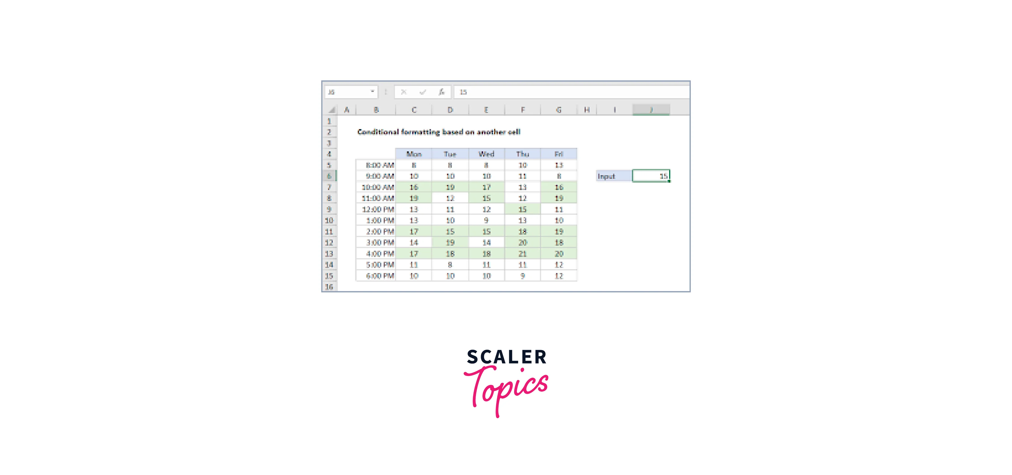
Excel Conditional Formatting Based on Another Cell

To apply conditional formatting in Excel based on the value of another cell, you can use a formula-based rule.

• Step 1: Select the cells or range of cells where you want to apply the conditional formatting.
• Step 2: Go to the "Home" tab in the Excel ribbon.
• Step 3: In the "Styles" group, click on the "Conditional Formatting" button. A dropdown menu will appear.
• Step 4: From the dropdown menu, select "New Rule." The "New Formatting Rule" dialog box will open.
• Step 5: In the "Select a Rule Type" section, choose "Use a formula to determine which cells to format."
• Step 6: In the "Format values where this formula is true" box, enter the formula that refers to the other cell.
• For example, if you want to highlight cells in column B if the corresponding value in column A is greater than 5, you can enter the formula: =$A1>5. Note that the "$" sign is used to lock the column reference (A) while allowing the row reference (1) to change as the conditional formatting is applied to different cells in the range.
• Step 7: Click on the "Format" button to specify the formatting style for the cells that meet the condition.
• Step 8: Choose the desired formatting options, such as font color, fill color, or cell borders.
• Step 9: Click "OK" to apply the conditional formatting rule.

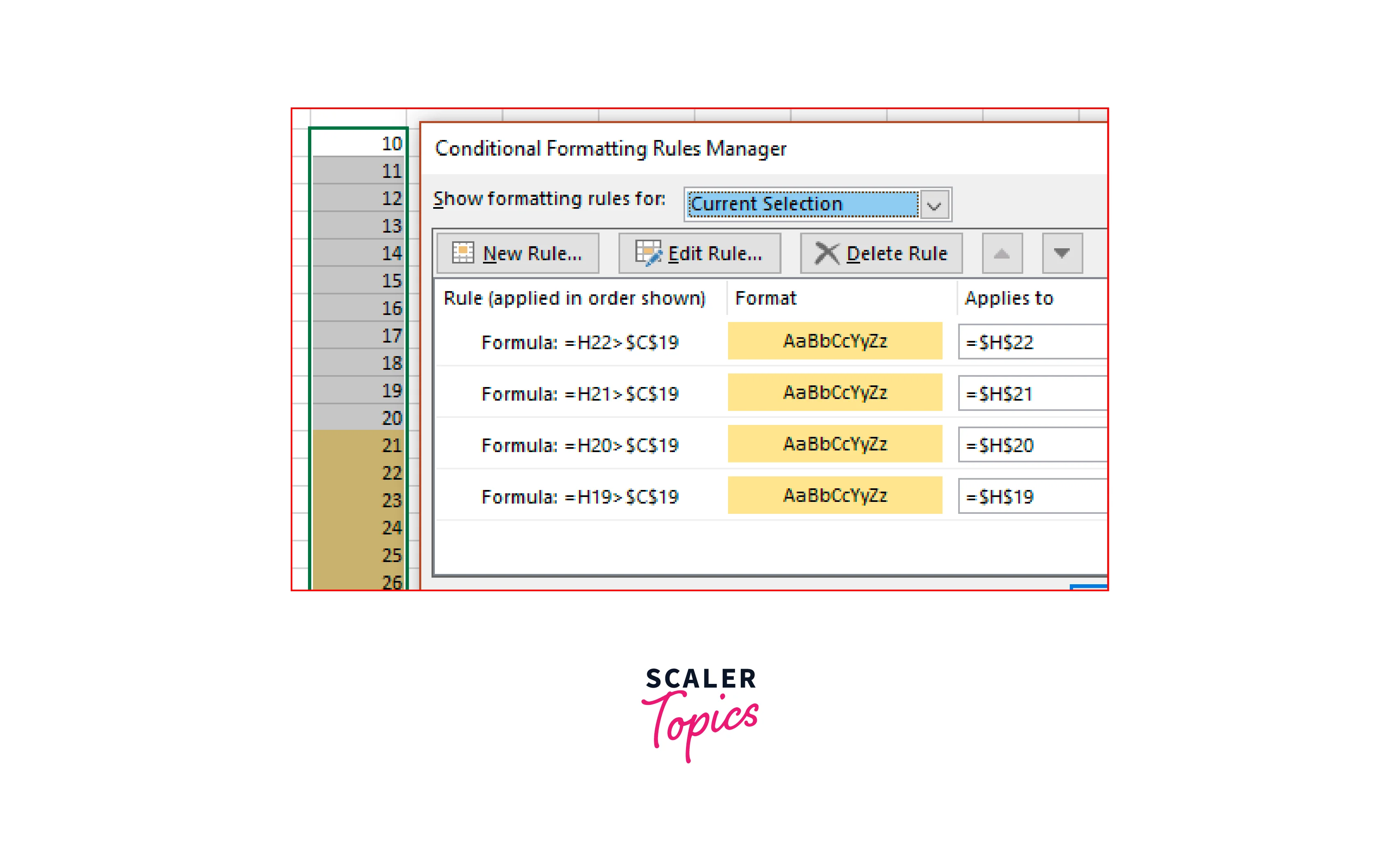
Multiple Conditional Formatting Rules to Same Cells

For applying multiple conditional formatting rules to the same cells in Excel. Each rule can have different criteria and formatting styles.

• Step 1: Select the cells or range of cells where you want to apply the conditional formatting.
• Step 2: Go to the "Home" tab in the Excel ribbon.
• Step 3: In the "Styles" group, click on the "Conditional Formatting" button. A dropdown menu will appear.
• Step 4: From the dropdown menu, select the desired type of conditional formatting rule. For example, you can choose "Highlight Cells Rules" or "New Rule."
• Step 5: Follow the steps to create the first conditional formatting rule based on your criteria and formatting preferences.
• Step 6: Once you have applied the first rule, go back to the "Conditional Formatting" button and select it again.
• Step 7: Choose another rule type or select "New Rule" to create a different rule.
• Step 8: Create the second conditional formatting rule based on different criteria and formatting options.
• Step 9: Repeat steps 6-8 if you want to add more rules.

Edit Excel Conditional Formatting Rules

To edit Excel conditional formatting rules refer to the steps below:

• Step 1: Select the cells or range of cells that have the conditional formatting rules you want to edit.
• Step 2: Go to the "Home" tab in the Excel ribbon.
• Step 3: In the "Styles" group, click on the "Conditional Formatting" button. A dropdown menu will appear.
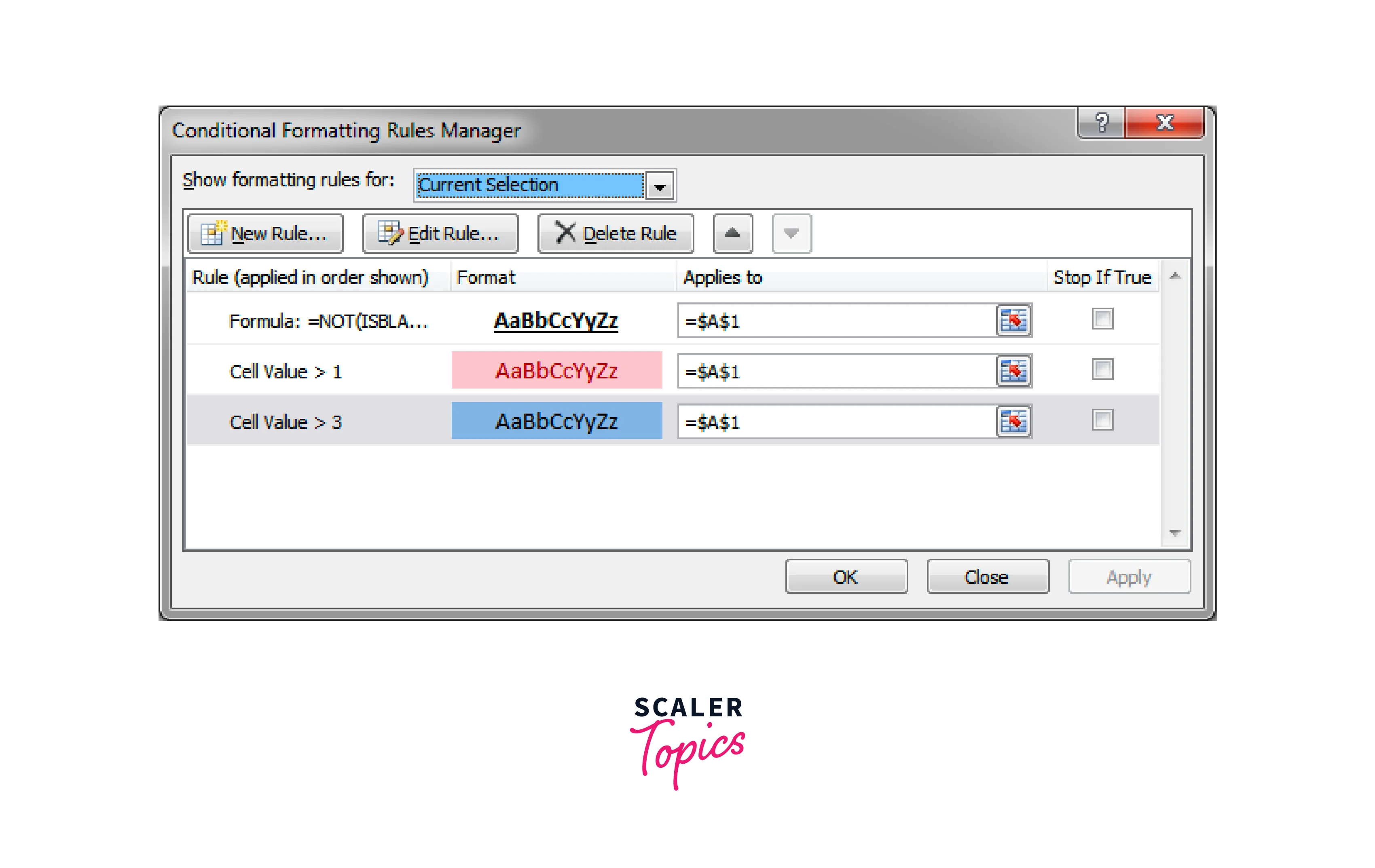
• Step 4: From the dropdown menu, select "Manage Rules." The "Conditional Formatting Rules Manager" dialog box will open.
• Step 5: In the "Conditional Formatting Rules Manager" dialog box, you will see a list of all the applied rules for the selected cells.
• Step 6: Select the rule you want to edit.
• Step 7: Click on the "Edit Rule" button on the right side of the dialog box.
• Step 8: The "Edit Formatting Rule" dialog box will open, allowing you to modify the criteria and formatting options for the selected rule.
• Step 9: Make the necessary changes to the rule, such as adjusting the formula, criteria, or formatting style.
• Step 10: Click "OK" to save the changes and update the conditional formatting rule.
• Repeat steps 6-10 if you want to edit additional rules.

Copy Excel Conditional Formatting

To copy conditional formatting from one cell or range to another in Excel, you can use the Format Painter tool.

• Step 1: Select the cell or range of cells that have the conditional formatting you want to copy.
• Step 2: Go to the "Home" tab in the Excel ribbon.
• Step 3: In the "Clipboard" group, click on the "Format Painter" button. The cursor will change to a paintbrush.
• Step 4: Click and drag the paintbrush cursor over the cell or range of cells where you want to apply the conditional formatting.
• Step 5: Release the mouse button. Excel will apply the copied conditional formatting to the selected cell or range.
• The Format Painter tool allows you to quickly copy the formatting, including conditional formatting, from one cell or range to another.

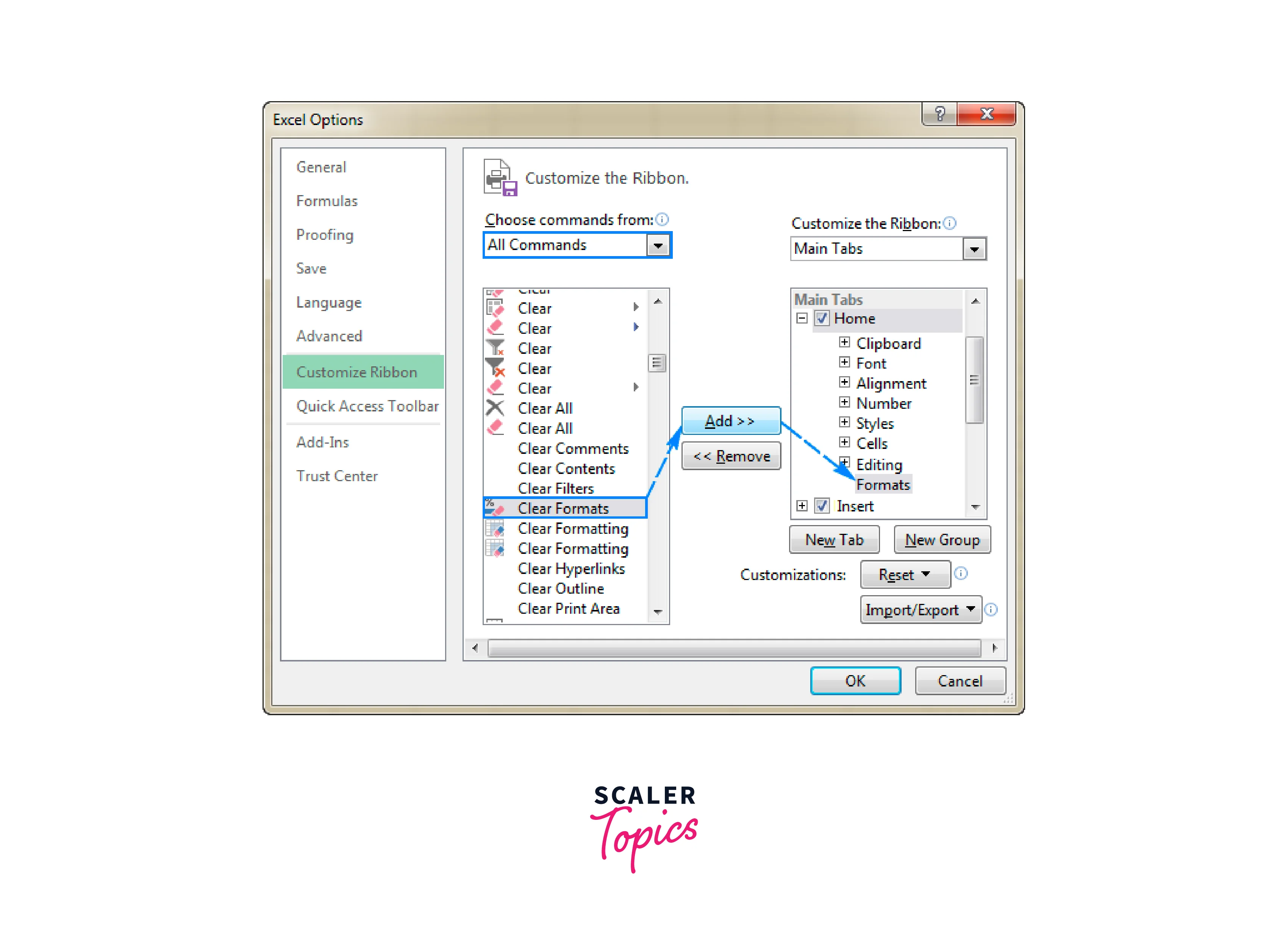
Clear Formatting

Clearing formatting in Excel is a useful feature that allows you to remove all formatting applied to cells, restoring them to their default appearance. It is particularly handy when you want to start with a clean slate or when you need to remove unwanted formatting from your spreadsheet. Clearing formatting ensures that your data is presented uniformly and consistently. Here's how you can use the "Clear Formatting" feature in Excel:

• Select the range of cells from which you want to clear the formatting. You can choose a single cell, a range of cells, or an entire worksheet.
• Go to the "Home" tab in the Excel ribbon. In the "Editing" group, you'll find the "Clear" button. Click on the small arrow next to it to open the dropdown menu.
• In the dropdown menu, select "Clear Formats" or "Clear All Formats." The option might vary slightly depending on the version of Excel you're using.
• Excel will remove all formatting applied to the selected cells, including font styles, font colors, cell colors, borders, number formats, and conditional formatting.

The "Clear Formatting" feature offers several benefits:

• Consistency:

  Clearing formatting ensures that all cells have a uniform appearance, making your spreadsheet look professional and organized. It eliminates any accidental or unwanted formatting, such as inconsistent font styles or colors, that may have been applied during data entry.

• Readability:

  By removing unnecessary formatting, you enhance the readability of your data. Clearing formatting can make your text easier to read by eliminating distracting font styles, sizes, or colors that might hinder comprehension.

• Formatting Troubleshooting:

  When encountering issues with formulas or data analysis, it's often beneficial to clear formatting to identify and troubleshoot problems. Formatting conflicts or incompatible formats can sometimes interfere with calculations or functions. By clearing formatting, you can isolate the issue and resolve it more effectively.

• Starting from Scratch:

  Clearing formatting is particularly helpful when you need to start with a clean slate. If you want to build a new spreadsheet or repurpose an existing one, removing formatting ensures that you're working with a fresh, unformatted sheet.

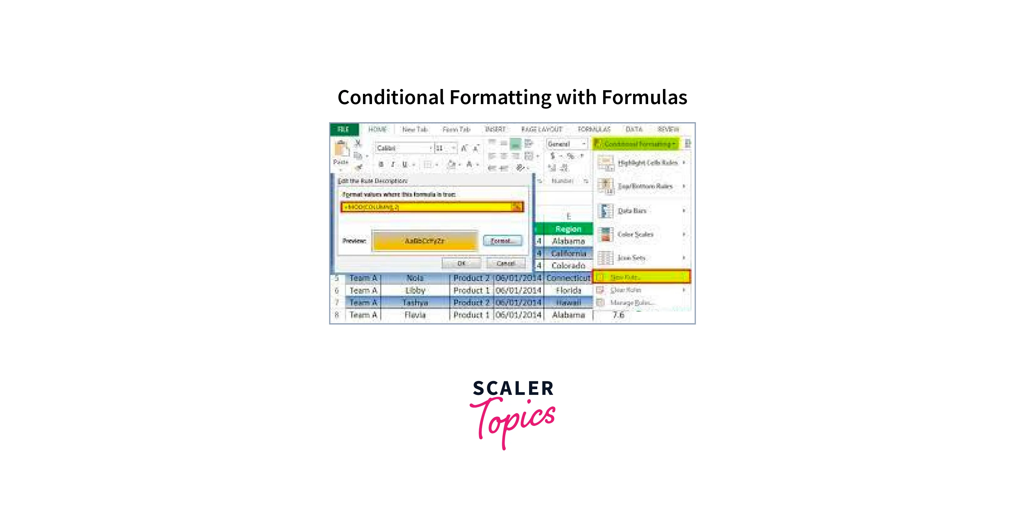
Conditional Formatting with Formulas

Conditional formatting with formulas is a powerful feature in Microsoft Excel that allows you to apply formatting to cells based on specific criteria defined by formulas. Unlike traditional conditional formatting, which relies on pre-defined rules, conditional formatting with formulas offers more flexibility and customization options.

Using conditional formatting with formulas, you can create complex rules to highlight cells, change font or background colors, add data bars or icon sets, and more, based on the results of the formulas. This allows for dynamic formatting that adapts to changes in the underlying data.

To apply conditional formatting with formulas, follow these steps:

• Select the range of cells you want to format.
• Go to the "Home" tab in the Excel ribbon and click on the "Conditional Formatting" button.
• Choose "New Rule" from the dropdown menu.
• In the "New Formatting Rule" dialog box, select "Use a formula to determine which cells to format".
• Enter the formula that evaluates to TRUE or FALSE to determine the formatting condition.
• Specify the formatting style or options you want to apply when the formula evaluates to TRUE.
• Click "OK" to apply the conditional formatting rule. For example, let's say you have a range of numbers in cells A1 to A10, and you want to highlight the cells that are greater than the average of the range. You can use the following formula in the conditional formatting rule:

This formula compares each cell in the range with the average of the entire range. If the cell value is greater than the average, the formula evaluates to TRUE, and the formatting will be applied.

Conditional formatting with formulas can be as simple or as complex as needed. You can use various functions, operators, and cell references within the formulas to define the conditions for formatting. This allows you to create rules based on specific numerical comparisons, text matching, date calculations, logical conditions, and more.

The real power of conditional formatting with formulas lies in its ability to handle dynamic scenarios. As your data changes, the conditional formatting is automatically updated based on the formula results. This ensures that your formatting remains consistent and reflects the latest values in the spreadsheet.

Furthermore, you can combine multiple formulas and conditions using logical operators like AND, OR, and NOT. This enables you to create sophisticated rules that consider multiple factors or dependencies.