What is CycleGAN and How it Works?

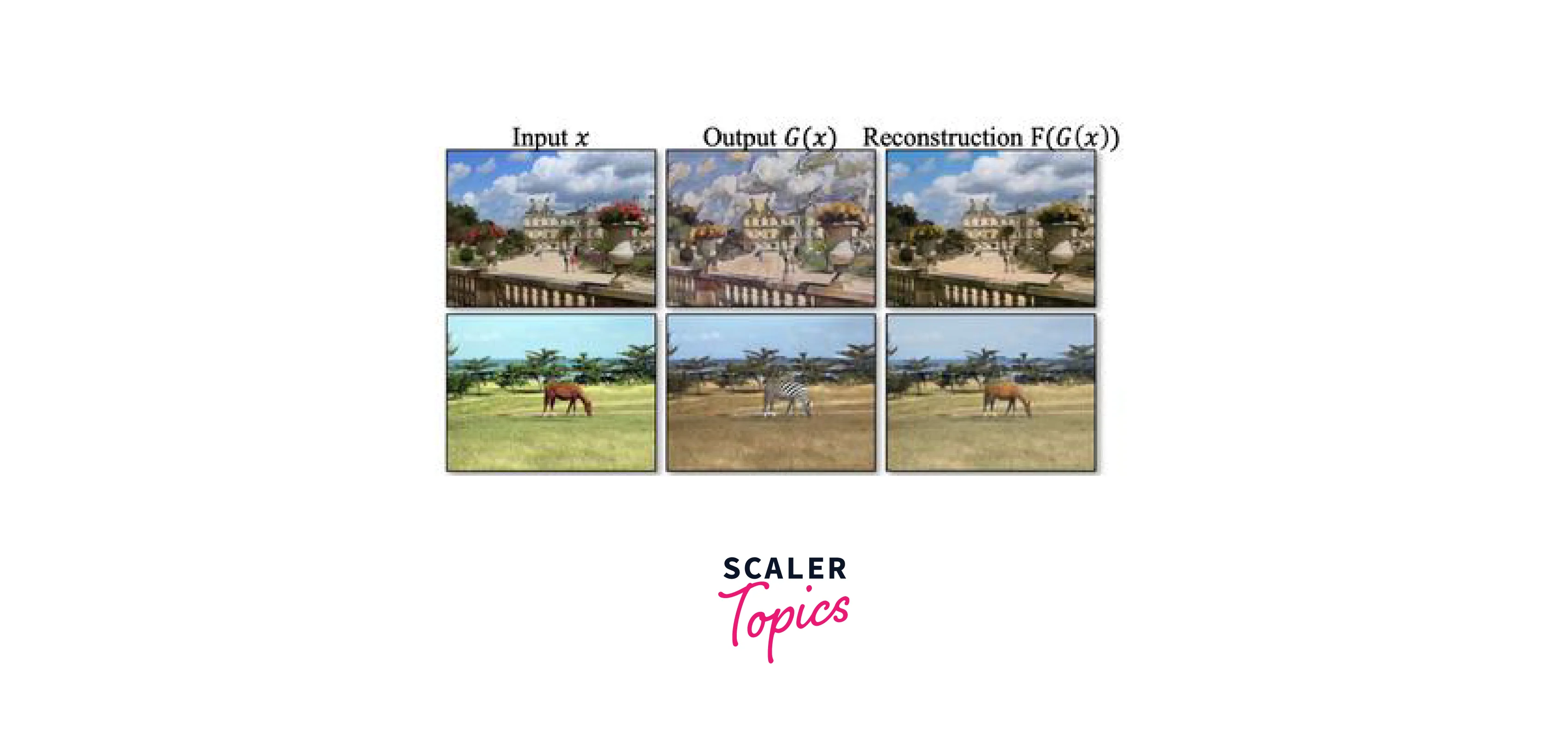
CycleGAN, an advancement from the Pix2Pix model, revolutionizes image-to-image translation without requiring paired datasets. Unlike Pix2Pix's constraint of needing matching images in both source and target domains, CycleGAN excels with unpaired datasets, enabling diverse tasks like translating RGB to SAR imagery or vice versa. This model's architecture employs dual generators and discriminators for bidirectional image conversion, extending its capabilities beyond Pix2Pix's limitations. Fundamentally, CycleGAN approaches image translation as a reconstruction challenge: an input image undergoes transformation by a generator to produce a new image, subsequently reversed to the original by another generator. The pivotal strength lies in its adeptness at unpaired image translation, where intrinsic relationships between input and output images aren't predefined, making it a potent tool for diverse image transformation tasks.

In this article, we will look at the internals of how to build such a GAN and cover the important implementational details theoretically.

An example of generated images is as follows.

How does CycleGAN Work?

This section details the inner workings of the CycleGAN and the components required to understand it. Since the CycleGAN is a rather complex model with many moving parts, it is important to understand the concepts behind Image2Image translation, the difference between paired and unpaired image data, and the main concept of adversarial training.

Architectural details such as a residual block, latent space, and a basic GAN are also summarized below.

Image2Image Translation

An image translation task aims to convert from one image to either text or another image. An example of the same would be as follows. Consider taking a picture of a sunset and converting that picture to the style of the artist Van Gogh. There are many such Image translation tasks. However, the task in consideration in this article is specifically converting from one image to another, aka Image2Image.

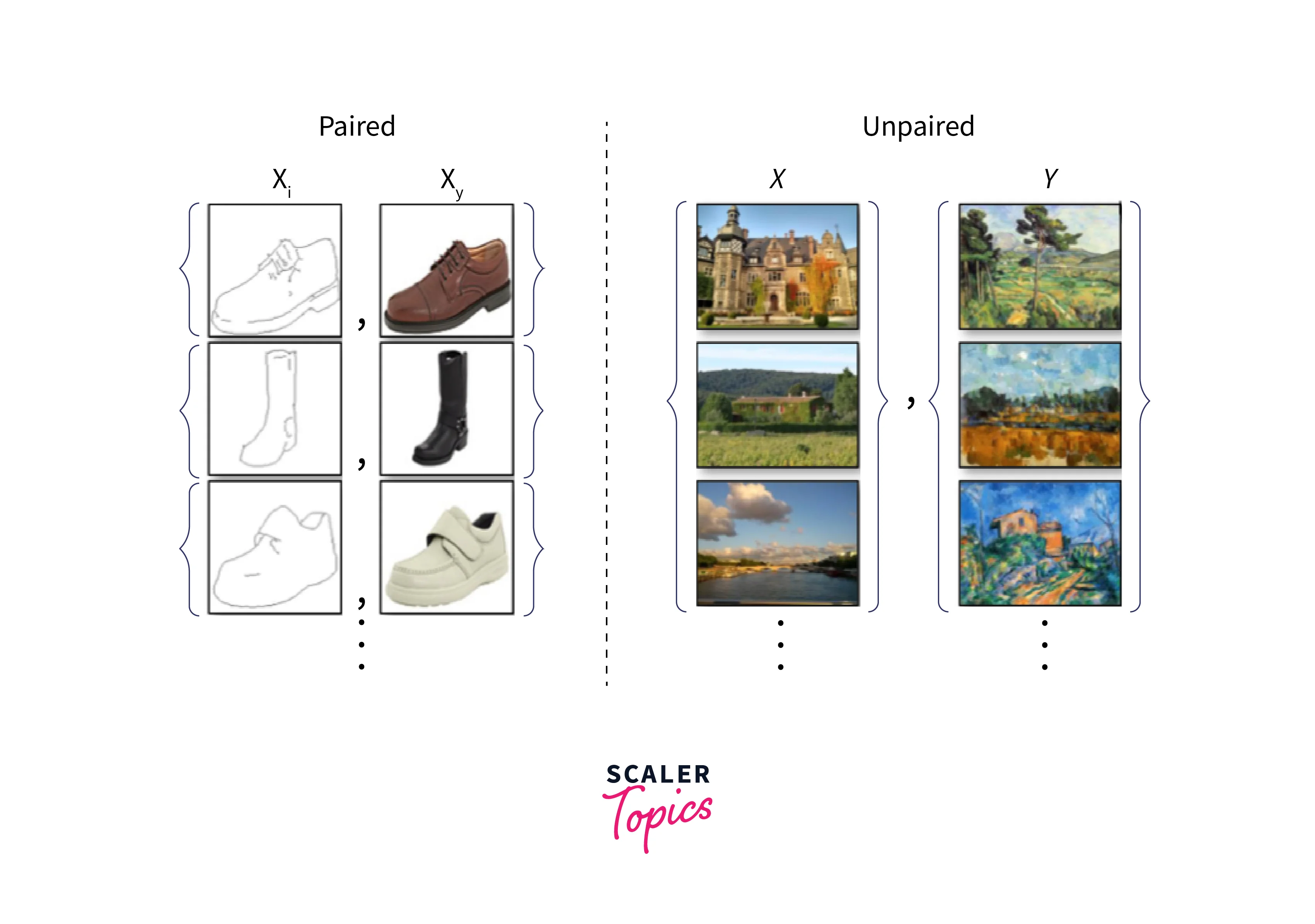
Paired vs. Unpaired Translation

An important detail about CycleGAN is that it uses an unpaired translation, unlike most other GANs or UNet-style architectures. This choice means that the image and label pairs passed to the model are unrelated. Contrary to say, a classification task where the label passed is the exact label of the image passed. This task might be clearer to understand with knowledge of latent space.

GAN

GANs are a special class of architectures with two components, one that tries to get better at a task and the other that determines how badly the first part performs. The training procedure is somewhat similar to a game, with one component being an "adversary" of the other, hence the term "Adversarial network". The generative term comes into play as these networks create novel images from existing data.

Adversarial Training

A useful analogy to understand how a GAN is trained is the classic "cop" vs. "thief" analogy. Assume that the thief, in this case, is trying to forge a painting by Van Gogh while the cop tries to prove the thief wrong. The thief first comes up with a forgery, and the cop says no, this is fake and not real for some reason. The thief then shows a modified image to the cop with minor differences. This scenario repeats until the cop can no longer distinguish between real and fake images.

This type of training is called adversarial training, where a second opinion is used to improve the outputs of the first component of the model. A good advantage here is that the data does not need to be labeled.

Residual Block

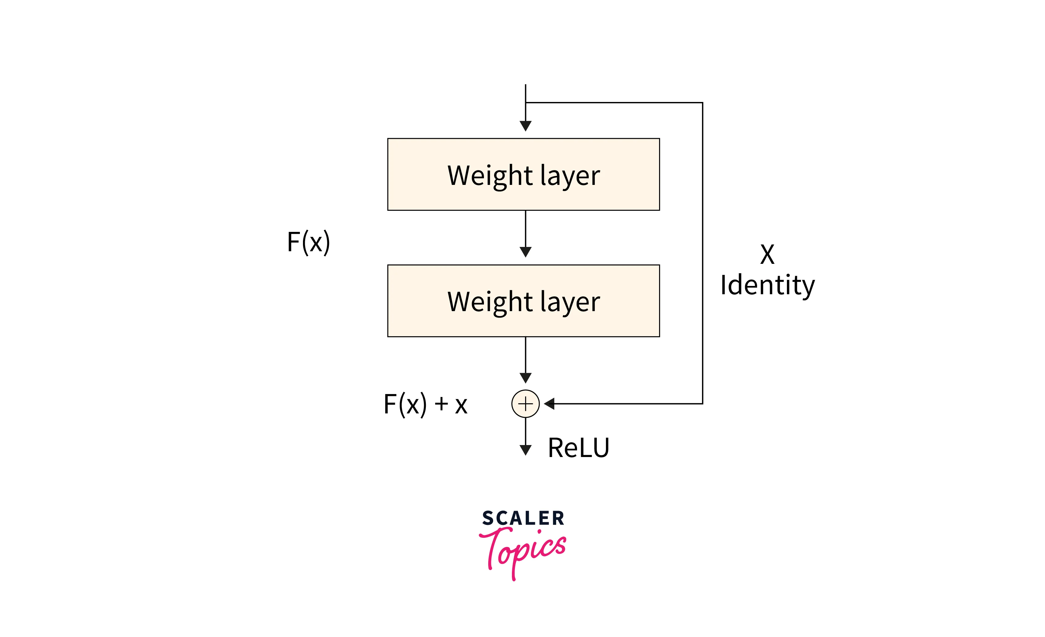
The Encoder-Decoder architecture has a major drawback; in compressing and reconstructing the image information, much information is lost during the operations. The Residual Block is the answer to this dilemma. It essentially contains a "Skip Connection" that ensures that the gradients from the previous layer are carried over to the next layer.

This connection is created very simply. If $F(x)$ is the network, then for an input $x_{i}$, $x_i = F(x_{i-1}) + x_{i-1}$.

Latent Space

Understanding latent space is the key to fully comprehending the CycleGAN. It is an n-dimensional vector space containing every possible image generated from the given data. Of course, it is only possible to visualize this partially, but a useful analogy is considering faces.

If we consider the faces of every person we know and "average" them together, we will end up with a "generic face" with traits from every face we consider. From this "generic face", if we were to attempt to recreate any of the other faces, we would have to "add" or "subtract" some features from the face to reach the other one.

This technique can be considered "traversing" the latent space. Thus, in essence, the latent space contains all such possible faces. In theory, it makes sense to assume that if we can approximate this latent space, we can translate any image to the other by traversing it. The CycleGAN attempts to do just that. Traversal can go in both directions. Hence it has a "cyclic" nature.

How is the Loss Calculated while Training?

CycleGAN uses a mix of three loss functions. Along with adversarial loss, a cycle consistency loss and an identity loss are used to create the final objective function.

Cycle Consistency Loss:

This loss function is the most important part of the CycleGAN research. Considering two image domains $X$ and $Y$ from the data, the Cycle consistency loss uses two different mappings $G: X \rightarrow Y$ and $F: Y \rightarrow X$. These mappings are bijections, aka reverses of each other. (Hence "cyclic"). As a mathematical expression, the Cycle Consistency Loss $\mathcal{L}_{cyc}$ can then be represented as $\mathcal{L}_{cyc}(G, F, X, Y) = \frac{1}{m}\Sigma_{i=1}^{m}[(F(G(x_{i})-x_{i})+ (G(F(y_{i}))-y_{i})]$.

Identity Loss:

Another loss function that CycleGAN proposes is Identity loss. $L_{identity}(G,F) = \mathbb{E}_{y \sim p_{data}(y)}[||G(y)-y)||_{1}] + \mathbb{E}_{x \sim p_{data}(x)}[||F(x)-x)||_{1}]$

This loss is especially useful for converting to and from photos and paintings. The loss is used to preserve the color information during transformation and to ensure that the reverse color is not used. If a part of the image looks like it belongs to the target image already, it is not mapped to something else. The model is more conservative if the transformed content is unknown.

Objective/Cost Function of CycleGAN

A cost function is an objective that the network tries to minimize. In essence, it is a metric of how well the network performs concerning a task. For example, for image classification, it could be CrossEntropy. CycleGAN has a rather complex cost function that is explained in later sections.

A hyperparameter $\lambda$ is used to control the strength of the transfer. It is usually set to 10. Therefore, the net loss function is a combination of all the described losses.

$\mathcal{L}_{GAN}(G, F, D_{X}, D_{Y}) = \mathcal{L}_{GAN}(G, D_{Y}, X, Y) + \mathcal{L}_{GAN}(F, D_{X}, X, Y) + \lambda \mathcal{L}_{cyc}(G,F)$

Thus, the function we wish to solve is finding the optimal optimizers' value that gives the best loss. We also want to maintain the ability to convert to and from the target image. To ensure these constraints, we use the formula.

$G^{*},F^{*} =\underset{G,F}{argmin} \underset{D_{X}, D_{Y}}{max} \mathcal{L}_{GAN}(G, F, D_{X}, D_{Y})$

CycleGAN Model Architecture

The CycleGAN architecture is divided into two major parts - The Generator and the Discriminator. The Generator has the Encoder, the Transformer, and the Decoder as components.

Encoder-Decoder Architecture

Many networks, such as the UNet and GANs, have a two-sided architecture that involves downsampling the image until a point and upsampling. The encoder is the first half that downsamples the image and condenses the information in a batch of data into the smallest possible unit. The decoder does the opposite; it takes the smallest possible unit and attempts to recreate the original input. In the process, it learns how to traverse the latent space and create the required translation. CycleGAN also follows this style of architecture. Understanding this point makes comprehending the model a lot simpler.

Generator Architecture

The Generator is the "thief". It starts with random noise to create a fake image and traverses the latent space until the Discriminator can no longer tell the difference between the fake and the real images. The Generator is grouped into the parts - Encoder, Decoder, and Transformer.

Encoder Block

The encoder uses convolution layers to consolidate information from the data and compress it into the least possible representational unit. The number of channels consequently increases. In the current model, there are three convolution operations. The final output of the model reduces the original image size by 3/4th and passes it to the Transformer Block.

"Transformer" Block:

The Transformer Block has nothing to do with "Transformer architectures" but is called so because it takes the output of the encoder and transforms it so the decoder can use it. This change ensures maximum information extraction from the encoder's compressed representation. In the CycleGAN, this block has around 6-9 Residual blocks.

Decoder Block:

The decoder block then takes the inputs from the transformer block and passes them through two de-convolution layers.

Discriminator Architecture

Consequently, the Discriminator is the "cop". The classifier returns a metric of the image's fake appearance. The Discriminator in the CycleGAN is another type of GAN - "PatchGAN". This special type of Discriminator uses input image patches to map to outputs. Unlike a normal GAN that maps from a $256x256$ sized image to a scalar result ("real" or "fake"), the PatchGAN maps it to NxN-sized arrays of outputs $X$ where each $X_{i,j}$ maps to ("real", "fake").

This part of the architecture is run as a convolution through the entire image, and the results are averaged.

Separate Optimisers

There are two optimizers for the Discriminator and the Generator each. (Four in total.) Using two different optimizers ensures that the model learns to convert images in both directions and minimizes the loss for both sets of generators and discriminators.

Instance Normalisation

Instance normalization is a technique that allows the network to remove specific contrast information when transferring style information between images. This technique makes CycleGANs extremely useful for image stylization tasks.

The formula is similar to Batch Normalisation and is left in this article as a reference.

Fractional Stride

Most networks use a stride that is a whole number. For example, CycleGAN has two types of convolutions. One type has a stride of 2, while the other has a stride of $\frac{1}{2}$. This stride is a special convolution case known as a "de-convolution". A fractional stride upsamples an image from a smaller dimension to a larger one. A whole number of stride downsamples it.

Reflection Padding

When performing convolutions, the sliding window does not always fit the size of the image to be convolved; padding is used in those cases to make up for the missing pixels. In CycleGAN, reflection padding is used, which means that the missing pixels are filled in with their neighboring pixels before being convolved instead of being filled with a "black" 0 pixel. This padding helps to preserve some more content information.

Applications of CycleGAN

As long as the dataset contains images in different folders with different painting style information alongside a folder of normal photos, CycleGAN can convert between them. This is called Unpaired Image to Image Translation..

The original paper has many such results. Some of these are shown below.

• Photos To Paintings:
  The procedure remains the same as before to convert photos to paintings with this network. The only difference is the dataset. We can apply a similar thought process to find other use cases, like converting photos to paintings. The ones that the paper mention are as follows :
• Style Transfer:
  Same as photos to and from paintings except with other types of imagery than just paintings.
• Object Transformation:
  Convert to and from objects within ImageNet classes by traversing the latent space. E.g., Converting apples to oranges, zebras to horses, and others.
• Season Transfer:
  Converting images from winter to summer and vice versa.

Strengths and Limitations of CycleGAN

CycleGAN has the following strengths:

• CycleGAN performs well for Image2Image tasks with style transfer elements.
• CycleGAN is bidirectional and can convert to and from the input and style images.

Some of the CycleGANs limitations are as follows:

• CycleGAN performs worse when given geometrical transformations.
• CycleGAN is trained to change appearances but does not penalize geometry changes. This design choice makes CycleGAN worse at preserving structure.

Implementation Tips for CycleGAN

CycleGAN has a complex implementation, and the authors mention a few required details.

• The Generator should have multiple Residual Blocks.
• The Discriminator should be a PatchGAN
• An additional 50 images are obtained by the Generator and fed into the Discriminator instead of the first batch generated.
• The Adam Optimizer with a small learning rate is to be used, with an initial pre-training for 100 epochs and a fine-tuning training for 100 more epochs with a decay in learning rate.
• The batch size is set to 1 to update the model after every image.