FP Growth Algorithm in Data Mining
Overview
The FP Growth algorithm in data mining is a popular method for frequent pattern mining. The algorithm is efficient for mining frequent item sets in large datasets. It works by constructing a frequent pattern tree (FP-tree) from the input dataset. FP Growth algorithm was developed by Han in 2000 and is a powerful tool for frequent pattern mining in data mining. It is widely used in various applications such as market basket analysis, bioinformatics, and web usage mining.
FP Growth in Data Mining
The FP Growth algorithm is a popular method for frequent pattern mining in data mining. It works by constructing a frequent pattern tree (FP-tree) from the input dataset. The FP-tree is a compressed representation of the dataset that captures the frequency and association information of the items in the data.
The algorithm first scans the dataset and maps each transaction to a path in the tree. Items are ordered in each transaction based on their frequency, with the most frequent items appearing first. Once the FP tree is constructed, frequent itemsets can be generated by recursively mining the tree. This is done by starting at the bottom of the tree and working upwards, finding all combinations of itemsets that satisfy the minimum support threshold.
The FP Growth algorithm in data mining has several advantages over other frequent pattern mining algorithms, such as Apriori. The Apriori algorithm is not suitable for handling large datasets because it generates a large number of candidates and requires multiple scans of the database to my frequent items. In comparison, the FP Growth algorithm requires only a single scan of the data and a small amount of memory to construct the FP tree. It can also be parallelized to improve performance.
Working on FP Growth Algorithm
The working of the FP Growth algorithm in data mining can be summarized in the following steps:
- Scan the database:
In this step, the algorithm scans the input dataset to determine the frequency of each item. This determines the order in which items are added to the FP tree, with the most frequent items added first. - Sort items:
In this step, the items in the dataset are sorted in descending order of frequency. The infrequent items that do not meet the minimum support threshold are removed from the dataset. This helps to reduce the dataset's size and improve the algorithm's efficiency. - Construct the FP-tree:
In this step, the FP-tree is constructed. The FP-tree is a compact data structure that stores the frequent itemsets and their support counts. - Generate frequent itemsets:
Once the FP-tree has been constructed, frequent itemsets can be generated by recursively mining the tree. Starting at the bottom of the tree, the algorithm finds all combinations of frequent item sets that satisfy the minimum support threshold. - Generate association rules:
Once all frequent item sets have been generated, the algorithm post-processes the generated frequent item sets to generate association rules, which can be used to identify interesting relationships between the items in the dataset.
FP Tree
The FP-tree (Frequent Pattern tree) is a data structure used in the FP Growth algorithm for frequent pattern mining. It represents the frequent itemsets in the input dataset compactly and efficiently. The FP tree consists of the following components:
- Root Node:
The root node of the FP-tree represents an empty set. It has no associated item but a pointer to the first node of each item in the tree. - Item Node:
Each item node in the FP-tree represents a unique item in the dataset. It stores the item name and the frequency count of the item in the dataset. - Header Table:
The header table lists all the unique items in the dataset, along with their frequency count. It is used to track each item's location in the FP tree. - Child Node:
Each child node of an item node represents an item that co-occurs with the item the parent node represents in at least one transaction in the dataset. - Node Link:
The node-link is a pointer that connects each item in the header table to the first node of that item in the FP-tree. It is used to traverse the conditional pattern base of each item during the mining process.
The FP tree is constructed by scanning the input dataset and inserting each transaction into the tree one at a time. For each transaction, the items are sorted in descending order of frequency count and then added to the tree in that order. If an item exists in the tree, its frequency count is incremented, and a new path is created from the existing node. If an item does not exist in the tree, a new node is created for that item, and a new path is added to the tree. We will understand in detail how FP-tree is constructed in the next section.
Algorithm by Han
Let’s understand with an example how the FP Growth algorithm in data mining can be used to mine frequent itemsets. Suppose we have a dataset of transactions as shown below:
| Transaction ID | Items |
| T1 | {M, N, O, E, K, Y} |
| T2 | {D, O, E, N, Y, K} |
| T3 | {K, A, M, E} |
| T4 | {M, C, U, Y, K} |
| T5 | {C, O, K, O, E, I} |
Let’s scan the above database and compute the frequency of each item as shown in the below table.
| Item | Frequency |
| A | 1 |
| C | 2 |
| D | 1 |
| E | 4 |
| I | 1 |
| K | 5 |
| M | 3 |
| N | 2 |
| O | 3 |
| U | 1 |
| Y | 3 |
Let’s consider minimum support as 3. After removing all the items below minimum support in the above table, we would remain with these items - {K: 5, E: 4, M : 3, O : 3, Y : 3}. Let’s re-order the transaction database based on the items above minimum support. In this step, in each transaction, we will remove infrequent items and re-order them in the descending order of their frequency, as shown in the table below.
| Transaction ID | Items | Ordered Itemset |
| T1 | {M, N, O, E, K, Y} | {K, E, M, O, Y} |
| T2 | {D, O, E, N, Y, K} | {K, E, O, Y} |
| T3 | {K, A, M, E} | {K, E, M} |
| T4 | {M, C, U, Y, K} | {K, M, Y} |
| T5 | {C, O, K, O, E, I} | {K, E, O} |
Now we will use the ordered itemset in each transaction to build the FP tree. Each transaction will be inserted individually to build the FP tree, as shown below -
-
First Transaction {K, E, M, O, Y}:
In this transaction, all items are simply linked, and their support count is initialized as 1.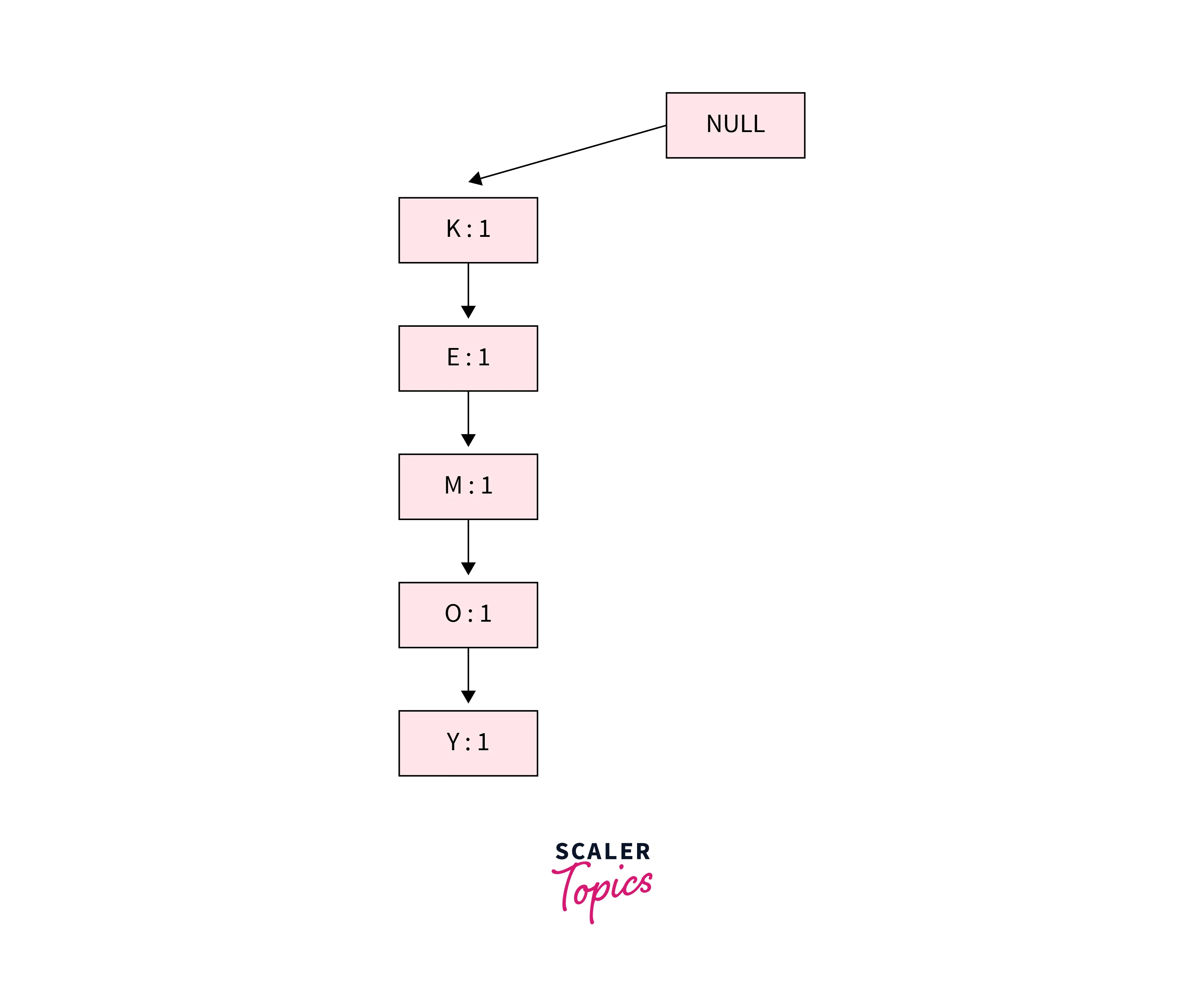
-
Second Transaction {K, E, O, Y}:
In this transaction, we will increase the support count of K and E in the tree to 2. As no direct link is available from E to O, we will insert a new path for O and Y and initialize their support count as 1.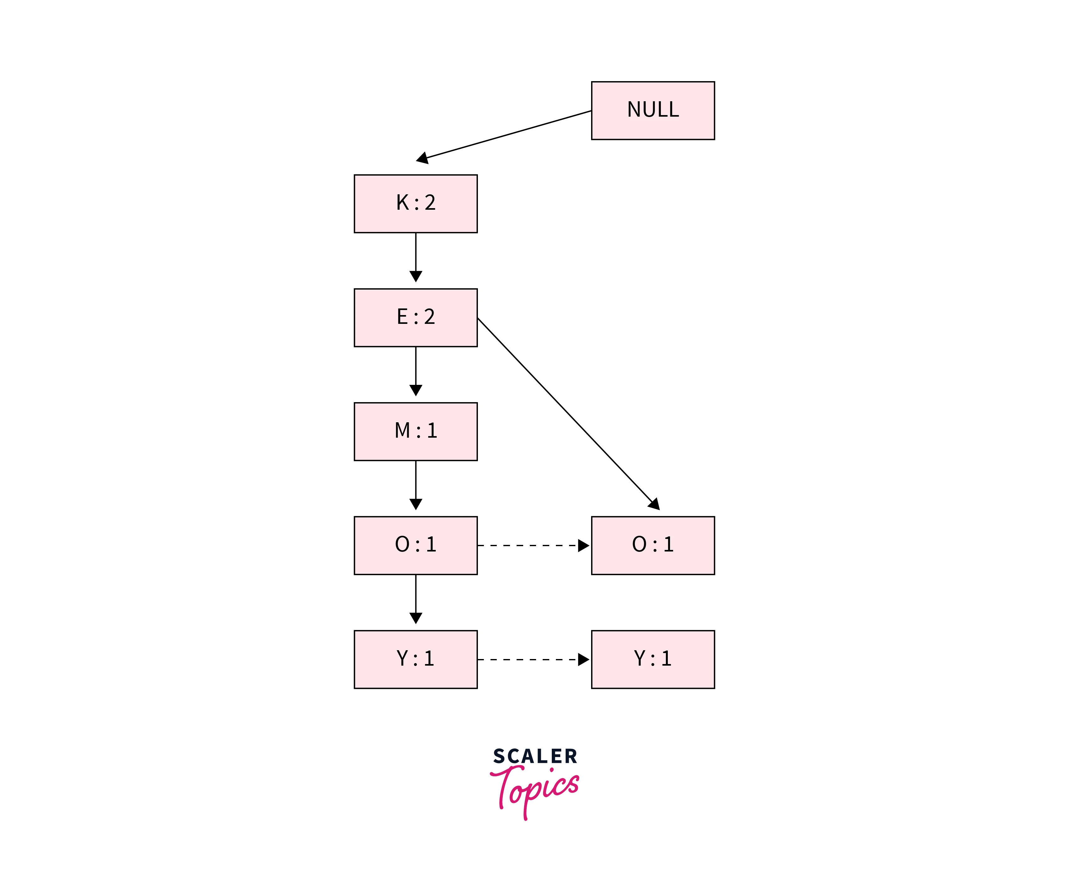
-
Third Transaction {K, E, M}:
After inserting this transaction, the tree will look as shown below. We will increase the support count for K and E to 3 and for M to 2.
-
Fourth Transaction {K, M, Y} and Fifth Transaction {K, E, O}:
After inserting the last two transactions, the FP-tree will look like as shown below: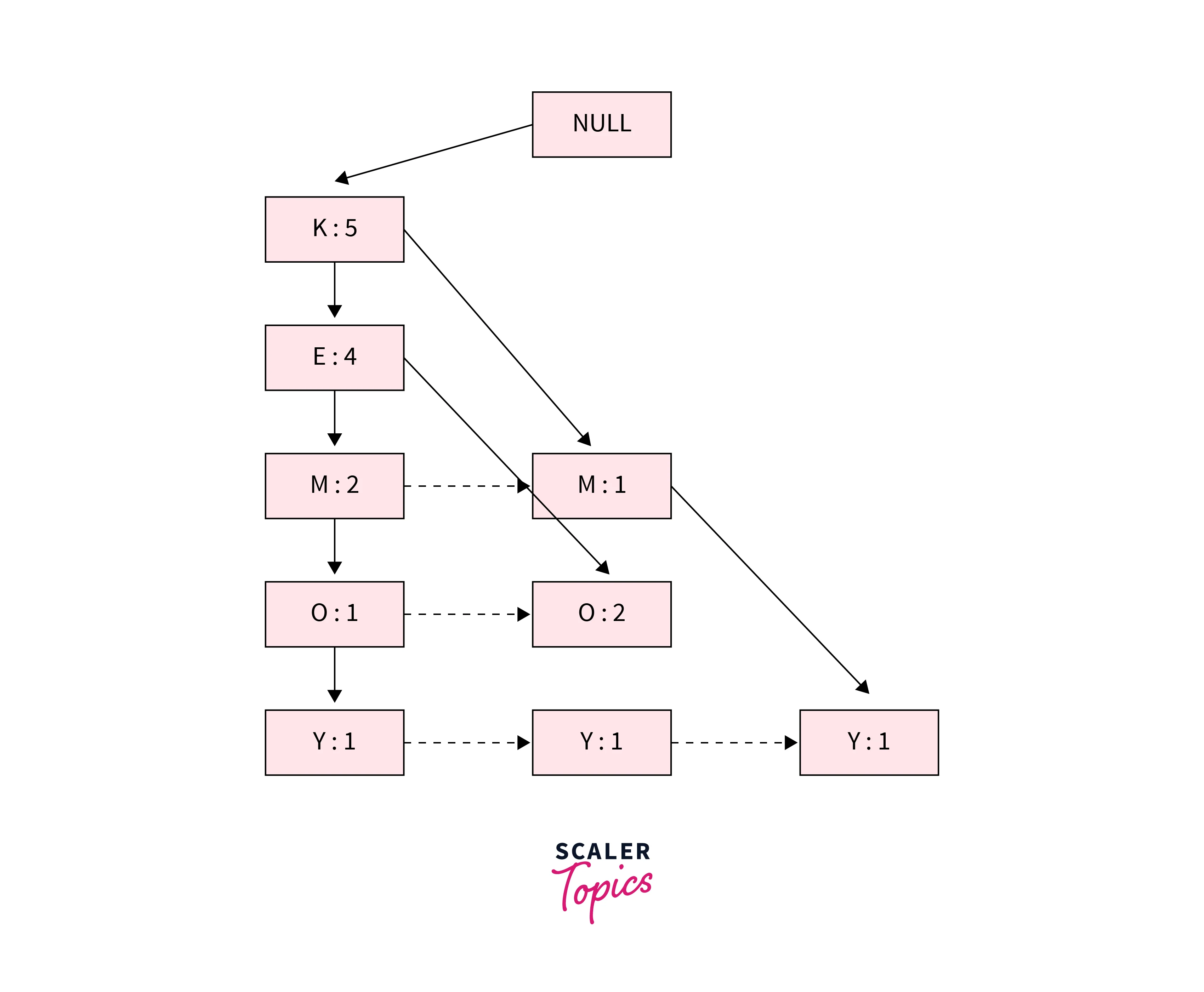
Now we will create a Conditional Pattern Base for all the items. The conditional pattern base is the path in the tree ending at the given frequent item. For example, for item O, the paths {K, E, M} and {K, E} will result in item O. The conditional pattern base for all items will look like as shown below table:
| Item | Conditional Pattern Base |
| Y | {K, E, M, O : 1}, {K, E, O : 1}, {K, M : 1} |
| O | {K, E, M : 1}, {K, E : 2} |
| M | {K, E : 2}, {K : 1} |
| E | {K : 4} |
| K |
Now for each item, we will build a conditional frequent pattern tree. It is computed by identifying the set of elements common in all the paths in the conditional pattern base of a given frequent item and computing its support count by summing the support counts of all the paths in the conditional pattern base. The conditional frequent pattern tree will look like this as shown below table:
| Item | Conditional Pattern Base | Conditional FP Tree |
| Y | {K, E, M, O : 1}, {K, E, O : 1}, {K, M : 1} | {K : 3} |
| O | {K, E, M : 1}, {K, E : 2} | {K, E : 3} |
| M | {K, E : 2}, {K: 1} | {K : 3} |
| E | {K: 4} | {K: 4} |
| K |
From the above conditional FP tree, we will generate the frequent itemsets as shown in the below table:
| Item | Frequent Patterns |
| Y | {K, Y - 3} |
| O | {K, O - 3}, {E, O - 3}, {K, E, O - 3} |
| M | {K, M - 3} |
| E | {K, E - 4} |
FP Growth Algorithm Vs. Apriori Algorithm
Here's a tabular comparison between the FP Growth algorithm and the Apriori algorithm:
| Factor | FP Growth Algorithm | Apriori Algorithm |
| Working | FP Growth uses FP-tree to mine frequent itemsets. | Apriori algorithm mines frequent items in an iterative manner - 1-itemsets, 2-itemsets, 3-itemsets, etc. |
| Candidate Generation | Generates frequent itemsets by constructing the FP-Tree and recursively generating conditional pattern bases. | Generates candidate itemsets by joining and pruning. |
| Data Scanning | Scans the database only twice to construct the FP-Tree and generate conditional pattern bases. | Scans the database multiple times for frequent itemsets. |
| Memory Usage | Requires less memory than Apriori as it constructs the FP-Tree, which compresses the database | Requires a large amount of memory to store candidate itemsets. |
| Speed | Faster due to efficient data compression and generation of frequent itemsets. | Slower due to multiple database scans and candidate generation. |
| Scalability | Performs well on large datasets due to efficient data compression and generation of frequent itemsets. | Performs poorly on large datasets due to a large number of candidate itemsets. |
Advantages of FP Growth Algorithm
The FP Growth algorithm in data mining has several advantages over other frequent itemset mining algorithms, as mentioned below:
- Efficiency:
FP Growth algorithm is faster and more memory-efficient than other frequent itemset mining algorithms such as Apriori, especially on large datasets with high dimensionality. This is because it generates frequent itemsets by constructing the FP-Tree, which compresses the database and requires only two scans. - Scalability:
FP Growth algorithm scales well with increasing database size and itemset dimensionality, making it suitable for mining frequent itemsets in large datasets. - Resistant to noise:
FP Growth algorithm is more resistant to noise in the data than other frequent itemset mining algorithms, as it generates only frequent itemsets and ignores infrequent itemsets that may be caused by noise. - Parallelization:
FP Growth algorithm can be easily parallelized, making it suitable for distributed computing environments and allowing it to take advantage of multi-core processors.
Delve Deeper: Our Data Science Course is Your Next Step. Enroll Now and Transform Your Understanding into Practical Expertise.
Disadvantages of FP Growth Algorithm
While the FP Growth algorithm in data mining has several advantages, it also has some limitations and disadvantages, as mentioned below:
- Memory consumption:
Although the FP Growth algorithm is more memory-efficient than other frequent itemset mining algorithms, storing the FP-Tree and the conditional pattern bases can still require a significant amount of memory, especially for large datasets. - Complex implementation:
The FP Growth algorithm is more complex than other frequent itemset mining algorithms, making it more difficult to understand and implement.
FAQs
Q. What is the FP Growth algorithm in data mining used for?
A. The FP Growth algorithm in data mining is a frequent itemset mining algorithm used to discover frequently occurring patterns in large datasets. It is commonly used in data mining, machine learning, and business intelligence applications.
Q. What is the difference between the Apriori algorithm and the FP Growth algorithm?
A. The Apriori and FP Growth algorithms are frequent item set mining algorithms but use different approaches to generate frequent item sets. The Apriori algorithm generates frequent item sets by repeatedly scanning the dataset and pruning infrequent item sets. In comparison, the FP Growth algorithm constructs an FP-Tree data structure and generates frequent item sets by traversing the tree.
Q. How does the FP-Tree data structure work?
A. The FP-Tree data structure is a compressed representation of the input dataset used by the FP Growth algorithm. It consists of root, internal, and leaf nodes, each representing an item. The FP-Tree allows frequent item sets to be generated efficiently by storing the support counts of each item and the relationships between them.
Conclusion
- The FP Growth algorithm in data mining is a frequent itemset mining algorithm used to discover frequently occurring patterns in large datasets. It generates frequent itemsets efficiently by constructing an FP-Tree data structure that represents the input dataset and mining the tree for recurring patterns.
- FP Growth algorithm is faster and more memory-efficient than the Apriori algorithm but requires sorting the input dataset by item frequency.