Data Structures in C++

Overview
Data structures are a particular way of organizing, storing, and managing data. You can use data structures to store and retrieve data efficiently whenever needed. Various types of data structures are used for storing different types of data based on the specific use case. The type of data structure that you will use will depend on the application you’re using. All the data structures are designed to arrange the data to suit a specific purpose, and each has its own advantages and disadvantages.
What are Data Structures in C++?
Data is an elementary value or the collection of values. For example, the employee's name is the data about the employee. To store this data in such a way that it becomes easily and efficiently accessible, we use the data structures.
Data structures are a specific way or a format of organizing data so that the information can be organized, processed, managed, stored, and retrieved quickly and effectively. They are a means of handling and rendering the data for easy use. The term data structure is mainly composed of Data and the various operations operating on that data. The data is the information, and the permissible operations are the algorithms working on that data to get valuable insights.
Data structures = Data + Permissible operations on that data
There are various types of data structures that you can use depending on your requirement, application, and use case. Choosing the right data structure according to the requirement is important so you can efficiently access the stored data. Each data structure has advantages and disadvantages, as each is designed to deal with a specific purpose.
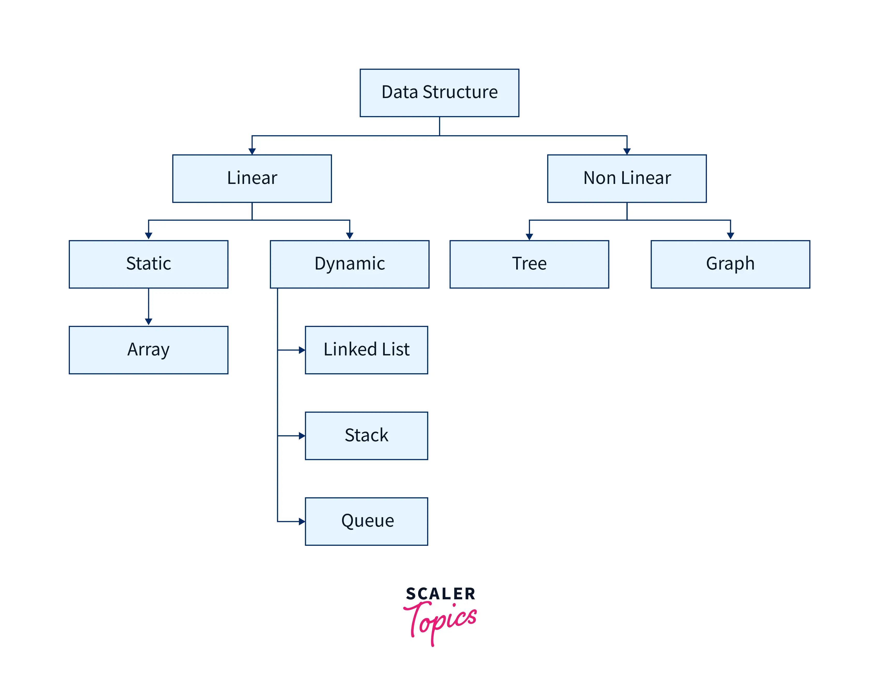
The data structures can be mainly classified into primitive and non-primitive data types, further into linear and non-linear data types.
Primitive Data Structures
Primitive data structures are one of the kinds of data structures that store data of only one type. They are the fundamental building blocks of data structures. The primitive data structures are the pre-defined data structures storing the data of only one data type. Some examples of primitive data types are integer, float, long, double, char, boolean, short, and byte. The four main types of primitive data structures available in all the programming languages are integer, float, boolean (true or false), and character.
The programming language already defines primitive data structures, or we can say that they are built-in data types in the programming languages.
Non-Primitive Data Structures
The non-primitive data structure is another type of data structure that can store more than one type of data. Non-primitive data structures are derived from primitive data structures, which are the user-defined data structures capable of storing more than one type of data in a contiguous or random memory location. Some examples of non-primitive data types include Array, Linked list, stacks, queues, trees, and graphs.
Non-primitive data structures are more complicated and complex than primitive ones but are highly useful for real-life applications.
Types of Data Structures in C++
Simple Data Structures
The simple data structures are built on top of primitive data types to create higher-level data structures that store a wide range of data according to the use case. The most common example of simple data structures are arrays and linked lists. We will look at both of these data structures later in this article.
Compound Data Structures
The compound data structures are built on top of primitive and simple data structures, which may be linear or non-linear. Some compound data structures are restricted to a single data type, while others are a mixture of multiple data types. We can say that compound data structures can contain multiple elements. Let's look at the types of compound data structures, i.e., linear and non-linear data structures:
-
Linear Data Structure A linear data structure is a compound data structure in which elements are stored linearly or sequentially. Each element is connected to its previous and the next element. Linear data structures are easy to implement because the computer memory is arranged linearly. As the data is stored linearly, it can be accessed or traversed in a single run or a traversal. In the linear data structure, elements are present at a single level. Examples of linear data structures include arrays, stacks, queues, and linked lists.
-
Non-Linear Data Structure The non-linear data structure is a compound data structure in which elements are not stored linearly or sequentially. As we know, in linear data structures, the element is connected to two elements (it's previous and the next element), but in non-linear data structures, the element can be connected to more than two elements. Non-linear data structures are more complex to understand and implement than linear ones. The data herein is not stored linearly and cannot be accessed or traversed in a single run. In a non-linear data structure, elements are present at multiple levels. Examples of non-linear data structures include trees, graphs, and maps.
Static and Dynamic Data Structures
The static data structure is where the size is allocated at the compile time. Therefore, the maximum storage size is fixed. In dynamic data structures, the size is allocated at the run time. Therefore, the maximum size is flexible and be changed according to the user. You can expand or contract a dynamic data structure according to your needs during the run time. An example of a static data structure is an array, and a dynamic data structure is a linked list.
Advantages and Disadvantages of Static Data Structure
- Data structure size is fixed.
- Not flexible.
- Stack is used in memory.
- Less efficient than a dynamic data structure.
- No memory reuse.
- Overflow is not possible.
- Memory allocation is done during compile time.
Advantages and Disadvantages of Dynamic Data Structure
- Memory allocation is done during run execution.
- Heap is used.
- More efficient than a static data structure.
- Memory reuse.
- Overflow occurs.
- Data structure size is not fixed.
- More flexible than a static data structure.
Let's see the basic overview of some of the linear and non-linear data structures:
Arrays in C++
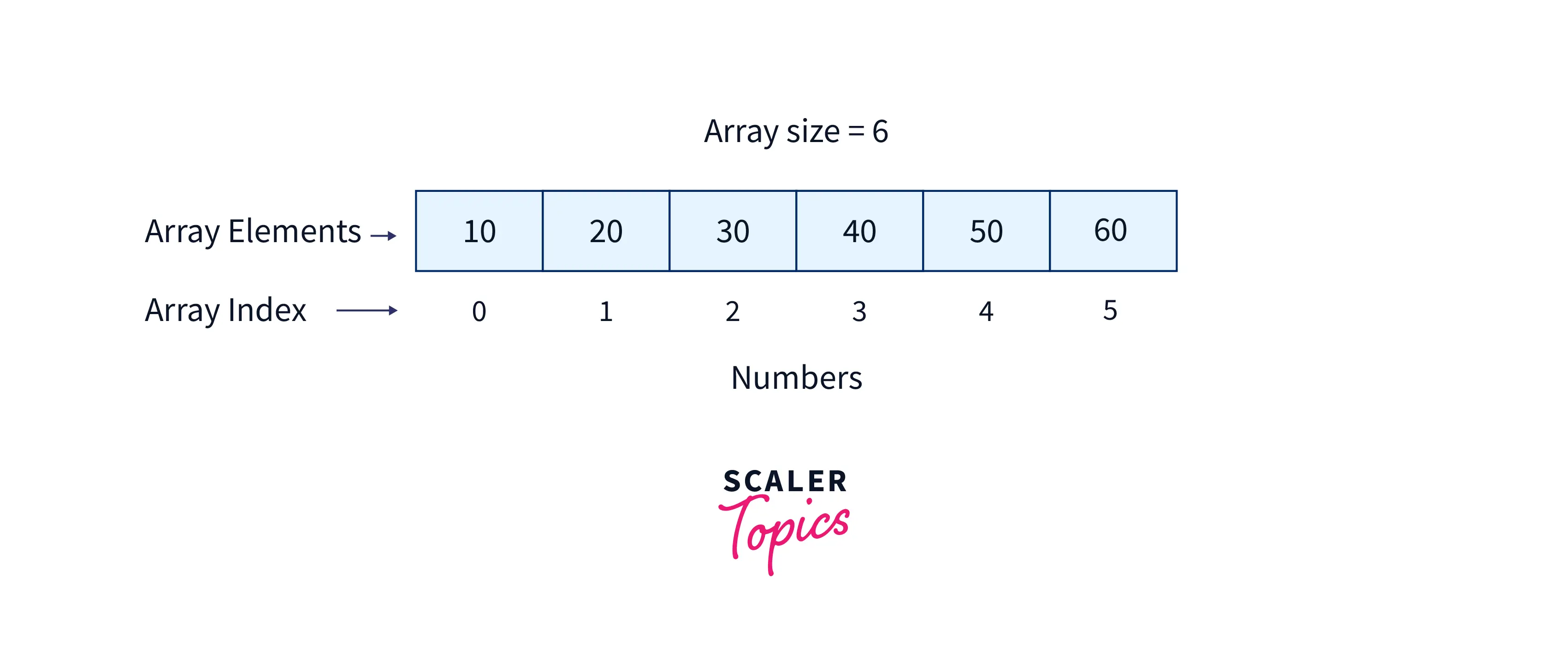
An array is a linear and sequential data structure having a fixed size. Arrays are the most basic, fundamental data structure, and they are usually present as a native data structure in many programming languages. It can hold items of the same data type, and each data item is known as an element of the array. The element's data type present in the array can be any valid data type like char, int, float, or double.
As arrays are indexed, random access is possible in arrays, and the indexing starts from 0.
The syntax for declaring the array is as follows:
We can assign the value at the specified array index using the syntax:
The value at any index present in the array can be retrieved using
To understand, like make an array of size 5 storing 5 integers: We can declare the array of fixed size 5 using the syntax:
Here, int is the data type of the elements stored in the array, and array is the array's name. To assign values in the array, we can write:
To return the value present at index 3, we can write:
The output of the above code would be 2, as the value stored at index 3 is 2.
Learn more about arrays in C++ from here
Strings in C++
The string data structure is an array or a group of characters. C++ has an inbuilt string class that can be used directly, or we can implement the arrays of characters to use a string data structure.
We can declare a string by declaring a one-dimensional array of characters. The only difference between a character array and a string is that a string is terminated with the null character \0.
We can declare the string in the same way we did for arrays, here the data type will always be the char of the elements stored in the string:
Here, char is the data type of the elements stored in the array, and stringArray is the array's name. To assign values in the array, we can write:
To return the value present at index 3, we can write:
The output of the above code would be 'l', as the value stored at index 3 is 'l'.
The character array will look like this:

Learn more about string in C++ from here
C++ Linked List
Linked list is a linear data structure, having a collection of nodes connected sequentially. Each node in a linked list consists of two components: the data or the value of that node and another is a pointer or link to the next node in the sequence. In a linked list, each node is only aware of the node next to it, so random index accessing is not possible in a linked list like arrays, so the concept of indexing is not valid in the case of a linked list.
There are mainly two types of linked lists: singly-linked lists and doubly-linked lists. A singly linked list is the most basic form of a linked list, where each node is only connected to the next node in the sequence. In a doubly-linked list, each node is connected to the node preceding and following it in the sequence.

As you can see from the image above, each node consists of a value and a link to the next node.
Learn more about linked list in C++ from here
Stack in C++
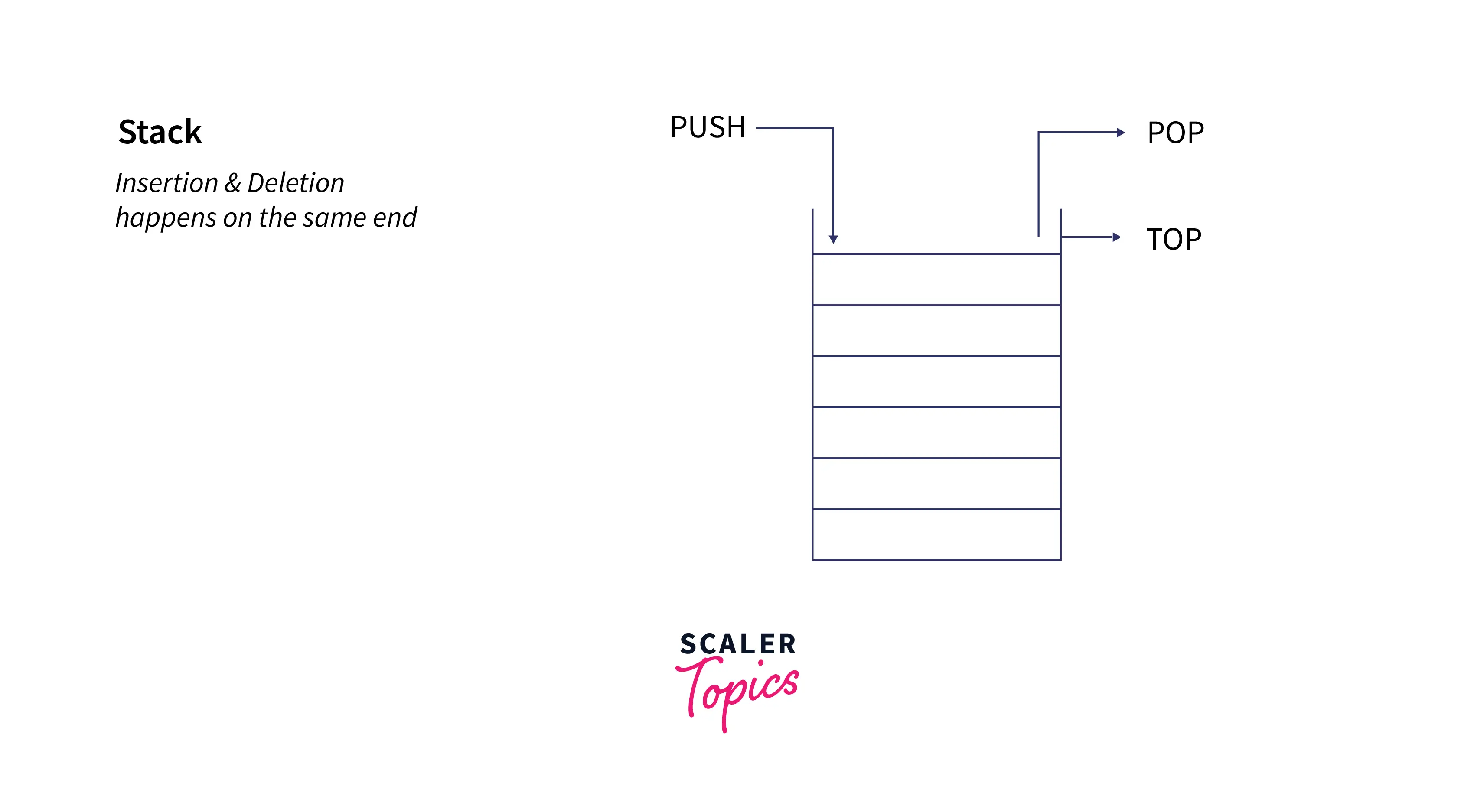
A stack is a linear data structure in which both the insertion and deletion operations occur only from a single end known as the top of the stack. Stack data structure follows the LIFO (Last In First Out — the element placed at last will be the one to be accessed at first) structure which means that we can only remove the most recently added item. The stack can be understood from a real-life example. It can be considered as a pile of plates or a deck of cards. The plate at the top will be the first one to be removed, and the plate placed at the bottom-most position will be the last one to be removed and will be the longer one to stay in the pile. Stack data structures have many applications. Because of their LIFO structure, they are the main mechanism supporting the “undo” or “back” button on many applications and browsers.
Some of the primary operations for stack include:
| Operation name | Operation Functionality |
|---|---|
| Push | adds an item to the stack |
| Pop | removes an item from the top of the stack |
| isEmpty | returns “true” on an empty stack and “false” if there is data present in the stack |
| isFull | returns “true” if the stack is full and “false” if the stack is not full |
| Peek or Top | returns the top element of the stack |
The time complexity of push(), pop(), isEmpty(), isFull(), and peek() all take O(1) time as we do not run any loop in any of these operations.
Learn more about stacks in C++ from here
Queue in C++
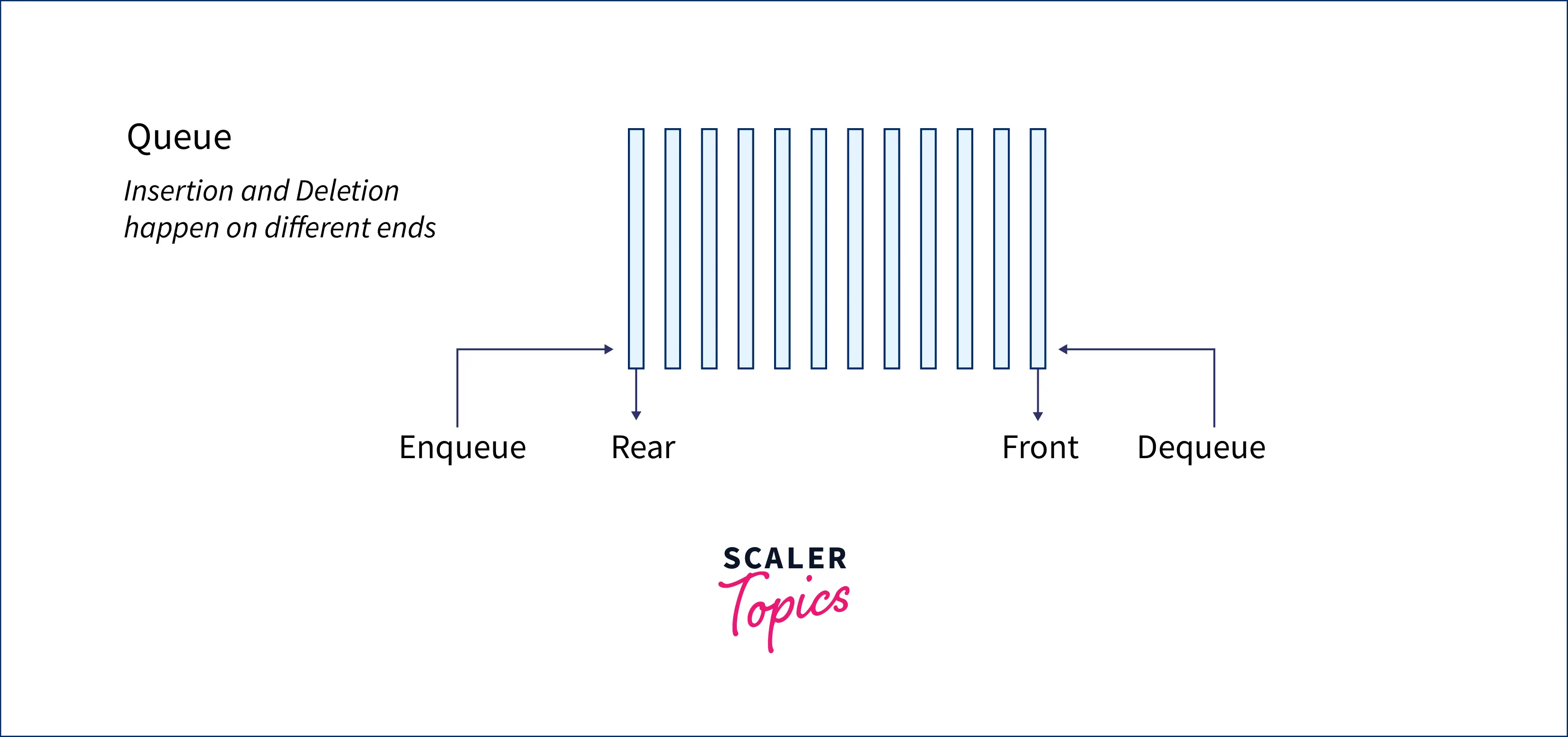
The queue is a linear data structure in which insertion and deletion operations occur from different ends. Queues follow FIFO (First In First Out — the element placed at last will be the last to be accessed, and the element placed in the starting will be the first to be removed) structure. The queue data structure can be understood from the real-life example as a queue of people at the ticket counter where the first person in the queue will be the one to get the ticket, and the last person in the queue will get the ticket in the last.
The difference between the stack and queue data structure is that the elements in the stacks are inserted and removed from the single end. Still, elements are inserted from the rear end in the queue while the elements are removed from the front end.
Some of the operations on the queue include::
| Operation name | Operation functionality |
|---|---|
| Enqueue | inserts an element in the rear or tail of the queue |
| Dequeue | removes an item from the front or head of the queue |
| isEmpty | returns “true” on an empty queue and “false” if there is data present in the queue |
| isFull | returns “true” if the queue is full and “false” if the queue is not full |
| Peek or Top | returns the front element of the queue |
The time complexity of all the operations is O(1) time, as we do not run any loop in any of these operations.
Learn more about queues in C++ from here
C++ Trees
The tree is a non-linear hierarchical data structure. Trees consist of nodes (i.e., vertices) and the edges that connect them. Each node has its data and the pointers that point to its parent node. There can only be one edge between two vertices, and the traversal usually occurs only in one direction, from the parent node to one of its children nodes (called "descendants"). The bottom nodes in the tree are called “leaf nodes,” while the topmost node is known as the “root node.” The leaf nodes do not have a child, and root nodes do not have parent nodes. The main application of a tree is to store hierarchical information, such as a file system.
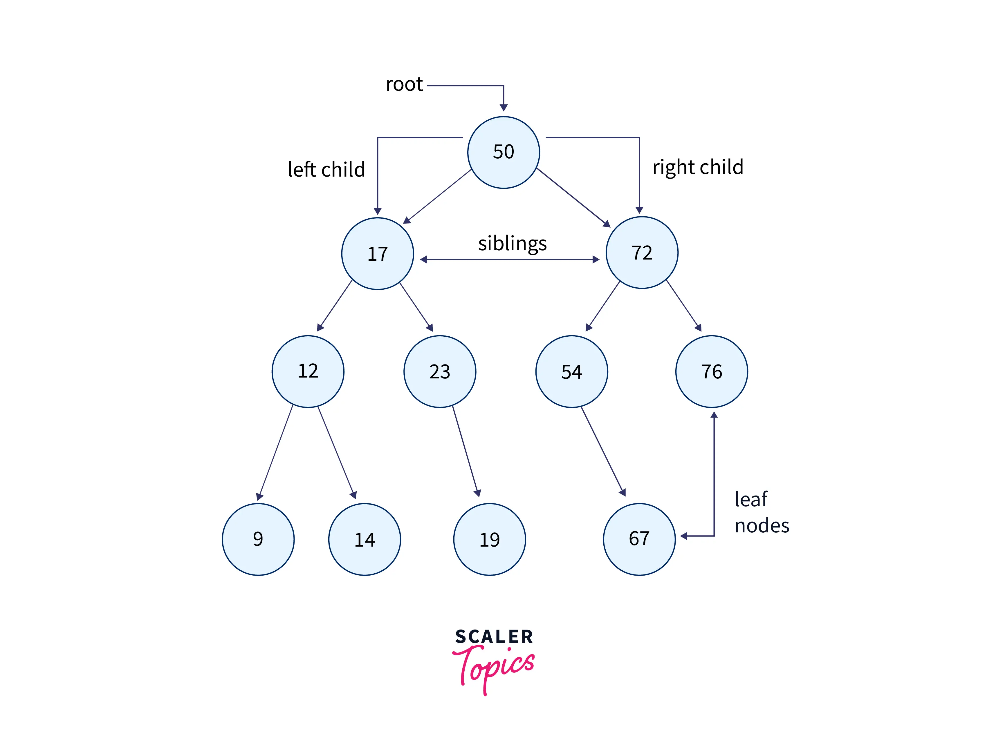
There are many types of trees, like binary trees, binary search trees, and tries. We will look at each of the types below:
Binary Tree
Binary trees are one type of tree data structure where each node has no more than two children, respectively called the right child and the left child. Each node in a binary tree has at most 2 child nodes.
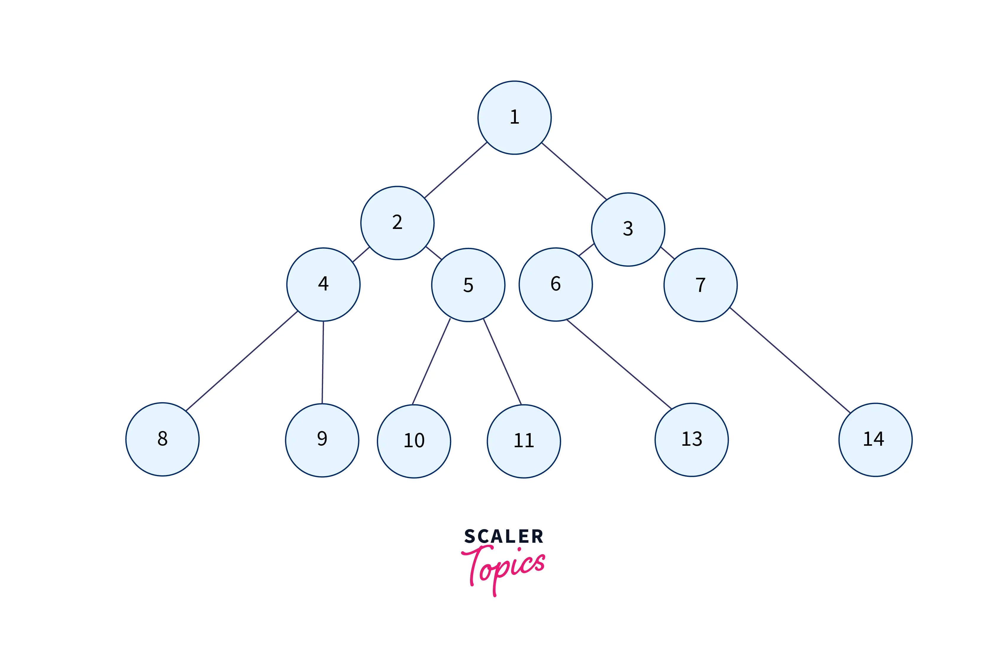
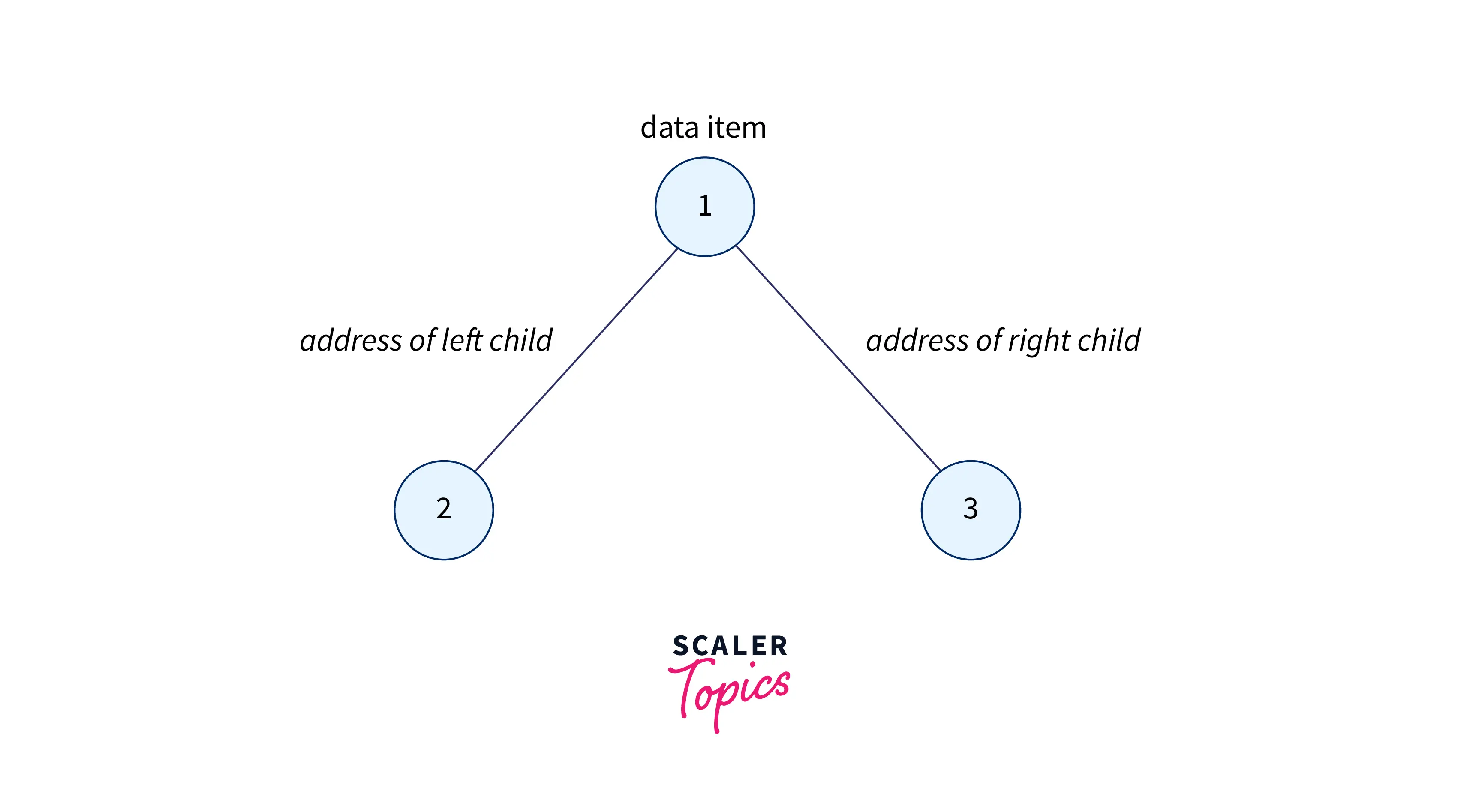
As we can see from the image above, each node in the binary tree has at most two child nodes (0, 1, 2 child nodes), and each node contains three parts, i.e., the data, the address, or the pointer to the left child, and a pointer to the right child as shown in the image below.
Learn more about binary trees from here
Binary Search Tree
A binary search tree is another type of tree data structure that follow some rules:
- The left subtree of a node contains only nodes with values lesser than the node’s key.
- The right subtree of a node contains only nodes with values greater than the node’s key.
- The left and right subtree must also be a binary search tree.
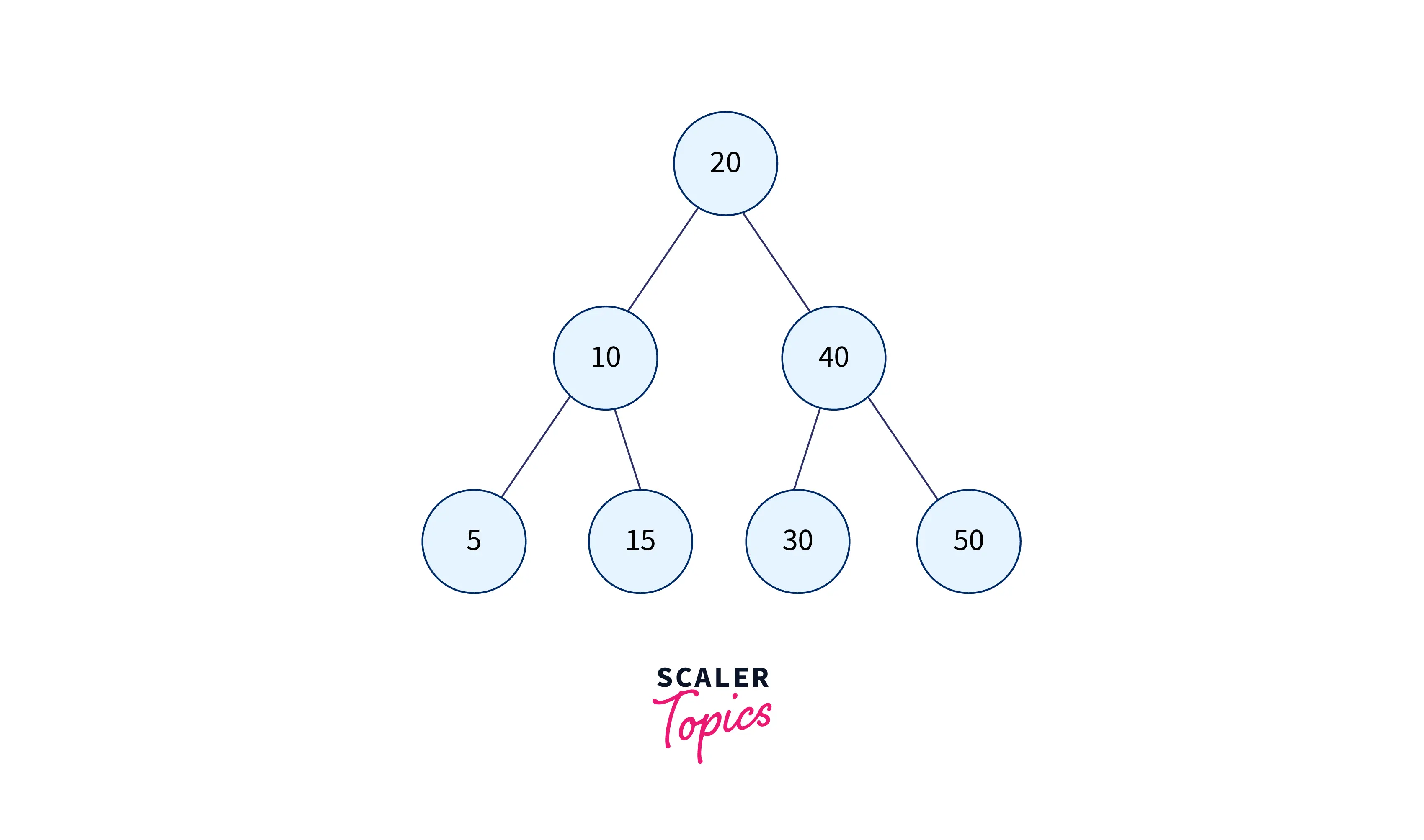
As you can see from the image below, each node on the left has a lesser value than the node's value, and each node on the right side has a greater value, and this pattern is recursively followed in the left and right subtrees.
A binary search tree allows quick lookup, add, and removal of data elements because of its pattern, and thus it also helps in the search algorithms.
Learn more about binary search trees from here
Tries
Tries are another type of tree data structure and are efficient data structures for solving programming problems involving strings. Tries consist of a collection of nodes, where each node represents a unique letter (trie can’t have duplicate nodes) of the alphabet, and the root node is the empty node that links to other nodes.
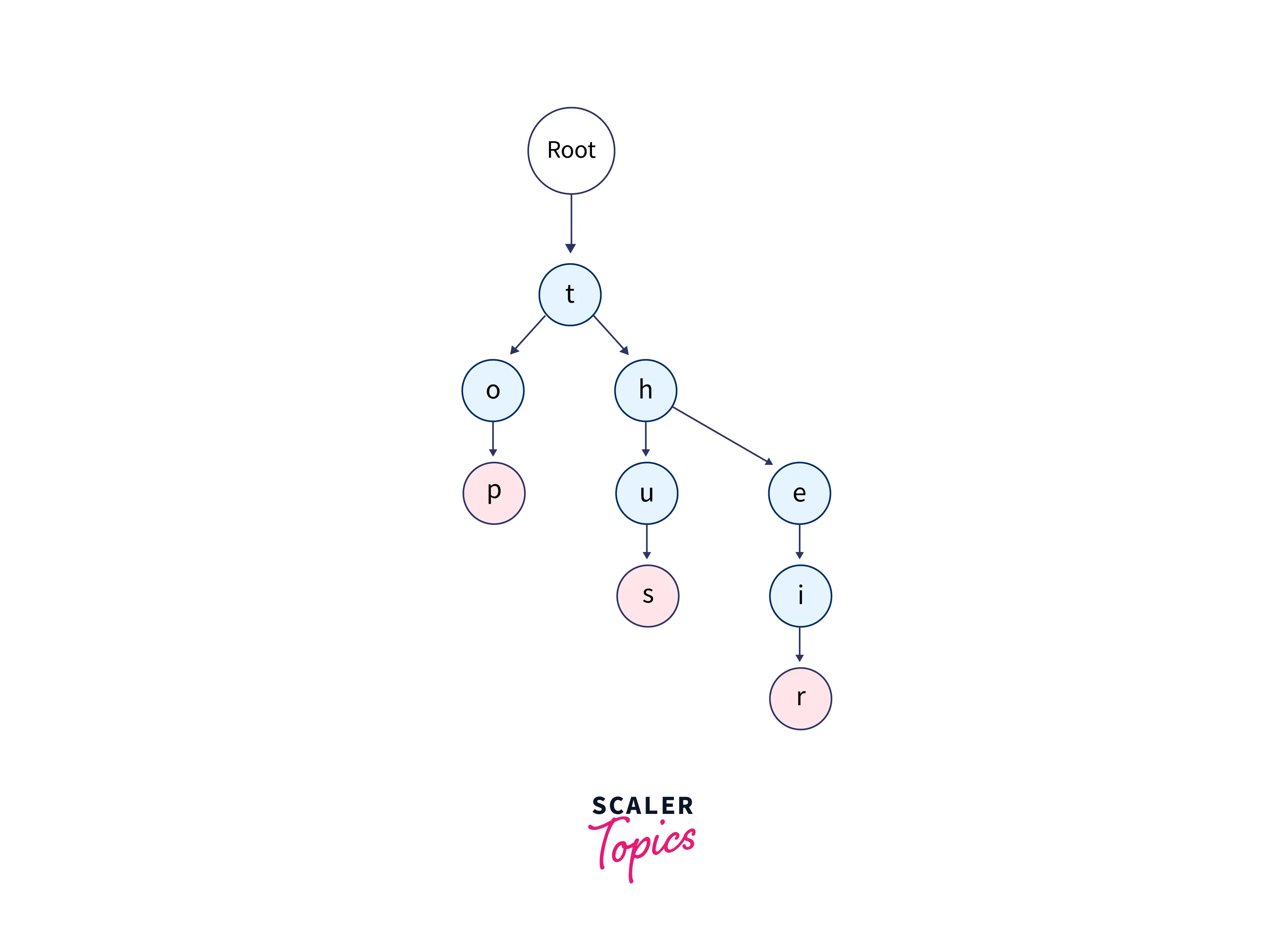
The diagram above shows a trie data structure with input strings as top, thus, and their. The root node represents an empty string.
Learn more about tries from here
Graphs
Graphs are non-linear data structures with finite nodes (sometimes called vertices) and edges. A graph differs from a tree as the graphs can have a cycle while the tree can not.
Graphs serve many real-life applications. They are used to represent networks. For example, on Facebook or Instagram, each person is represented with a vertex that contains information like person id, name, gender, etc., and persons or the nodes are connected via the edges.
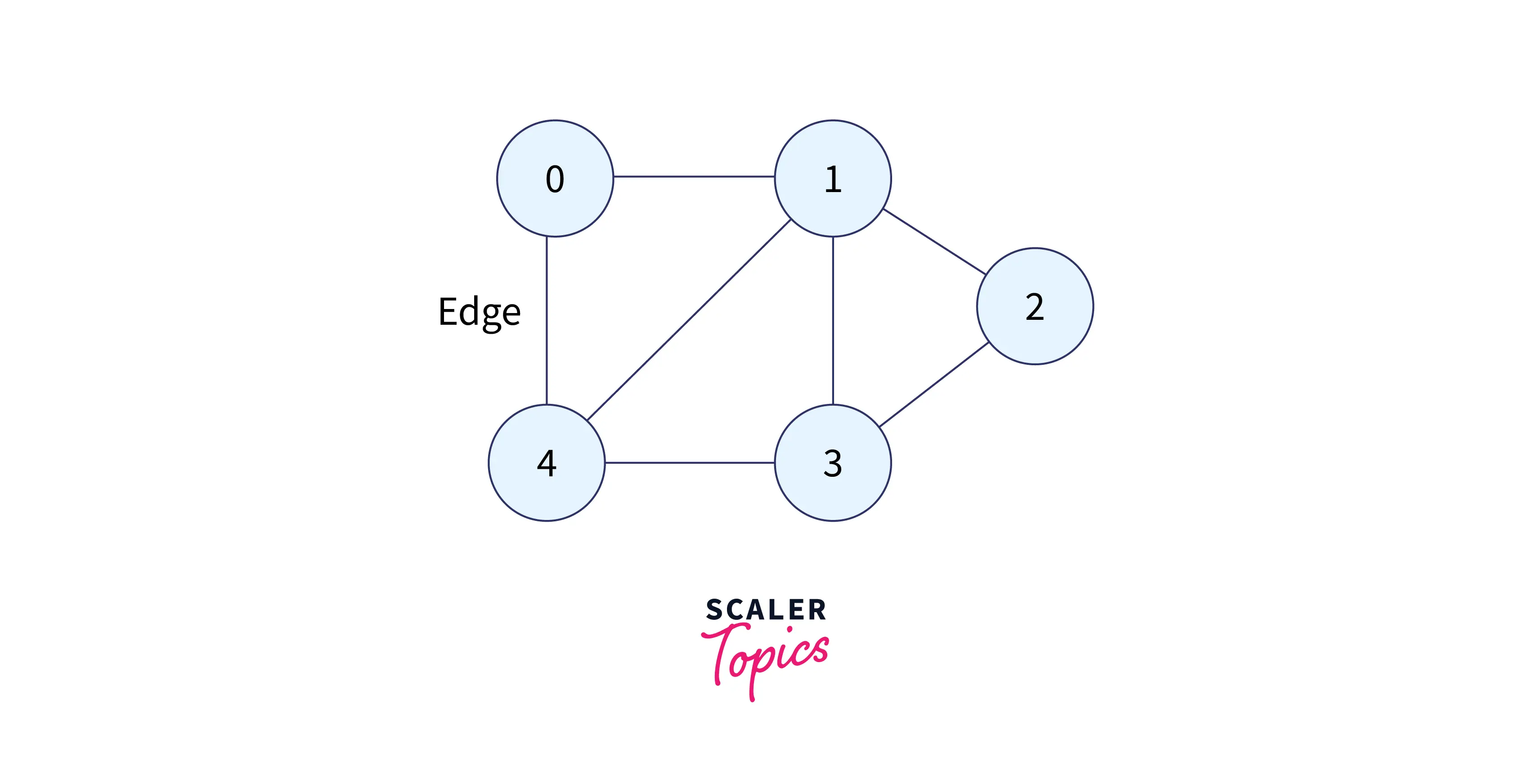
There are mainly three types of graphs:
- Undirected graphs: A graph in which all edges are bi-directional, and each edge can be traversed in both directions.
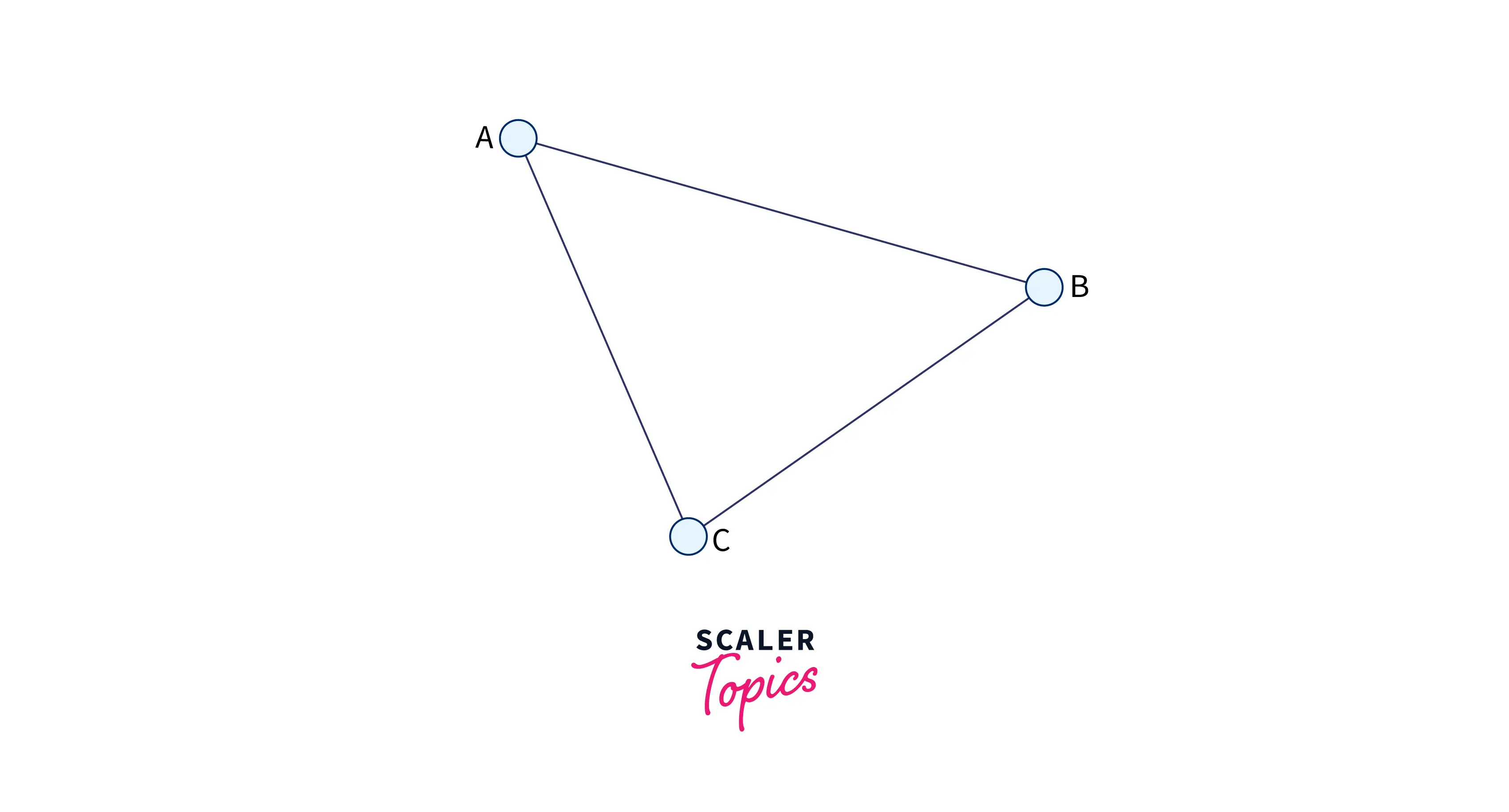
As we can see from the image above, we can traverse from A to B, B to A, A to C, C to A, B to C, and C to B.
- Directed graphs: A graph in which all edges are unidirectional, which means that each edge can only be traversed in a single direction.
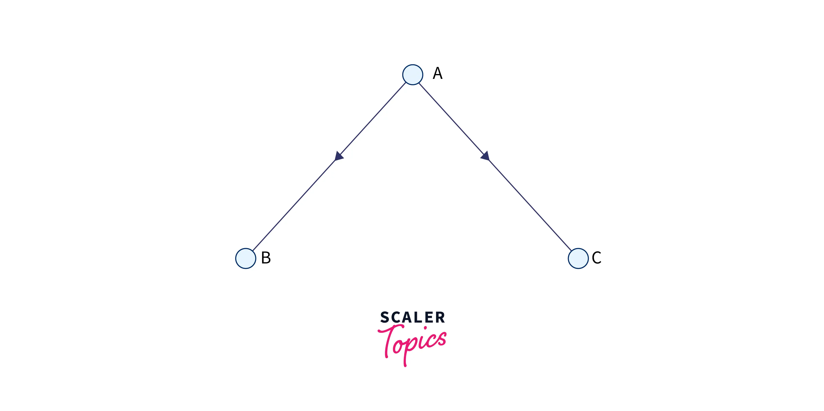
As we can see from the image above, we can traverse from A to B and A to C.
- Weighted graphs: A graph in which all edges are assigned a value (known as a weight).
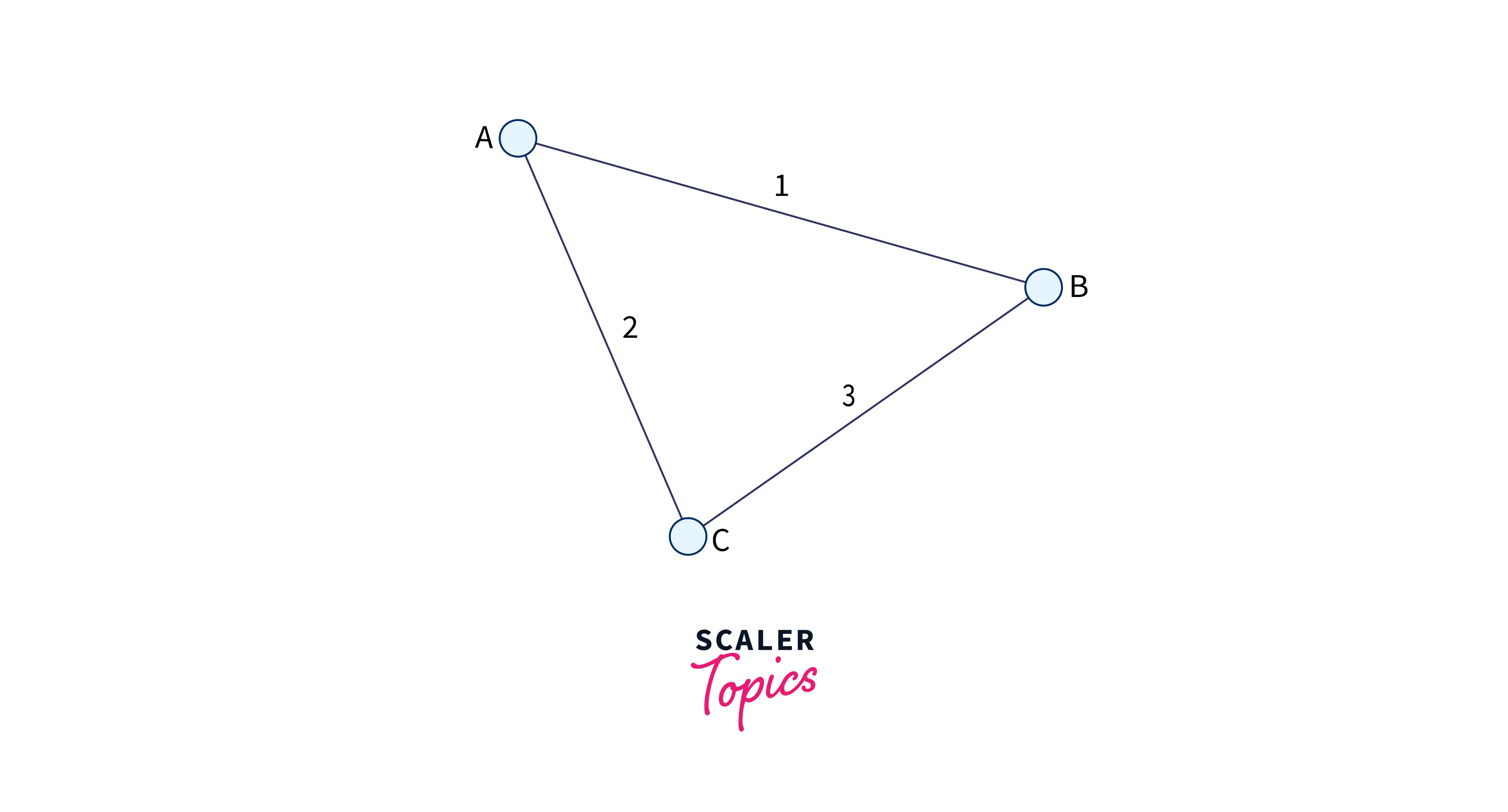
As we can see from the image above, the weight of the edge between A to B is 1, A to C is 2, and C to B is 3.
Learn more about graphs from here
Hash Table
Hash tables are also called hash maps. It stores the key (a unique integer used for indexing the values) and the corresponding value (data associated with the key). Here, each unique key is associated with the corresponding value, which can be retrieved by accessing the key.

We can access the value in a hash table by calling hashMapName[key], and the data will be returned as the output.
Accessing data is very fast in hash tables if we know the key of the desired data. Thus, it becomes a data structure where insertion and search operations are very fast and efficient, irrespective of the data size.
Learn more about hash tables from here
Conclusion
- Data structures are a specific way of organizing, processing and storing data such that it can be retrieved quickly and effectively. They are used to handle the information and the rendering of data.
- Data structures provide efficiency, reusability, and abstraction to the data.
- Primitive data structures store data of only one data type, whereas non-primitive data structures store data of multiple data types.
- In the linear data structure, elements are stored sequentially and linearly (Examples - arrays, stacks, queues, and linked lists), whereas in non-linear data structures, elements are not stored linearly or sequentially (Examples - graphs, trees).
- Arrays are a linear data structure storing a collection of elements of the same data type placed in contiguous memory locations.
- String is a group or a collection of characters.
- Linked list is a linear data structure consisting of nodes containing a data field and a pointer to the next node in the sequence.
- Stack is a linear data structure that follows the LIFO (Last In First Out) structure, and the queue is also a linear data structure that follows FIFO (First In First Out).
- Tree is a non-linear, hierarchical data structure consisting of vertices and edges.
- Binary tree is one of the types of tree data structure where each node must have at most two child nodes, known as the left and the right child
- Binary search tree is a tree in which each node has a value greater than the nodes on its left side and a value lesser than the nodes on its right side.
- Trie is an ordered tree data structure that stores strings to solve complex problems involving strings.
- Graph is a complex non-linear data structure having a finite set of nodes and edges. Three common types of graphs are undirected, directed, and weighted.
- Hash table is a data structure that allows us to store, retrieve, and delete data uniquely based on their unique key.
