Data Wrangling in R Programming

Need of Data Wrangling

Data wrangling is essential for several reasons. Some of these are:

1. Data Formatting for Analysis:

• The primary purpose of data wrangling is to ensure that the data is in a suitable format for analysis. Raw data is often messy and comes from various sources, leading to inconsistencies in its structure.
• By employing data wrangling techniques in R, we can standardize the data, making it uniform and ready for further exploration.

2. Addressing Inconsistencies and Missing Values:

• Real-world data commonly contains inconsistencies and missing values, which can hamper the accuracy of analyses if left unaddressed.
• Data wrangling in R enables us to detect and handle these issues, ensuring that our data is complete and reliable.

3. Flawless Analysis and Modeling:

• Proper data wrangling practices in R significantly reduce the risk of flawed or inaccurate analyses.
• When data is meticulously prepared through wrangling, the results of subsequent analyses and modeling are more trustworthy and robust.

4. Improved Data Quality and Reliability:

• Data wrangling contributes to enhancing the overall quality and reliability of the data.
• By cleaning and transforming the data, we can eliminate errors and inconsistencies, thus producing higher-quality datasets.

5. Facilitating Data Integration:

• In data science projects, data is often gathered from diverse sources, leading to varying formats and structures.
• Data wrangling in R helps streamline the integration process, harmonizing the data into a unified format for seamless analysis.

6. Enabling Efficient Data Exploration:

• Unwieldy and unprocessed data can hinder the exploration of valuable insights.
• Through data wrangling, we can organize and structure the data, facilitating a more efficient exploration of its patterns and relationships.

7. Preparing for Data Visualization:

• Effective data visualization requires well-structured data that can be easily interpreted and plotted.
• Data wrangling in R sets the stage for meaningful data visualizations by transforming the data into a suitable format.

8. Ensuring Compliance and Data Privacy:

• In certain domains, data privacy and compliance regulations necessitate careful data handling and cleansing.
• Data wrangling allows us to anonymize or pseudonymize sensitive information, ensuring adherence to data protection regulations.

Data Import

Before we can start wrangling, we need to import the data into R. R offers numerous packages like readr and data.table, enabling us to efficiently read data from various file formats such as CSV, Excel, or databases. let's explore data import methods using different packages and formats:

1. Using readr Package for CSV Import:

The readr package provides efficient functions to read data from CSV files. Let's consider an example where we have a CSV file named "data.csv" containing the following data:

To import this data into R, we can use the read_csv() function:

Output:

2. Using readxl Package for Excel Import:

The readxl package allows us to read data from Excel files (.xlsx) easily. Let's assume we have an Excel file named "data.xlsx" with the following data in the "Sheet1":

To import this Excel data into R, we can use the read_excel() function:

Output:

3. Using data.table Package for Efficient Import:

The data.table package is known for its high-speed data manipulation capabilities. It offers fast data import functions like fread() for reading data from various file formats. Suppose we have a CSV file named "data_large.csv" with a large dataset:

Output:

4. Database Connectivity and Data Import:

In addition to file-based data import, R allows us to connect to databases and retrieve data directly. The RSQLite package is one such example that enables access to SQLite databases.

Suppose we have an SQLite database named "my_database.db" with a table named "mtcars":

Output:

Data Cleaning

Data cleaning is an integral aspect of data wrangling, ensuring the quality and integrity of data, thus setting the stage for precise and trustworthy analyses. By addressing missing values, eliminating duplicates, and managing outliers, we can enhance the quality of our datasets. Emphasizing data cleaning within the data wrangling process in R will ensure you're working with premium data, the cornerstone for insightful analyses and data-driven decisions

Now let's delve into the importance of data cleaning and explore various techniques to handle missing or erroneous data:

1. Handling Missing Values:

Missing values are a common occurrence in real-world datasets and can adversely impact the accuracy of our analyses. R provides several methods to handle missing values effectively. Let's consider an example with a vector containing some missing values:

Output:

2. Removing Duplicates:

Duplicates can skew our analysis results, leading to redundant information and potentially misleading insights. Data cleaning involves the identification and removal of duplicates to ensure data integrity. Let's demonstrate this with a data frame containing duplicate rows:

Output:

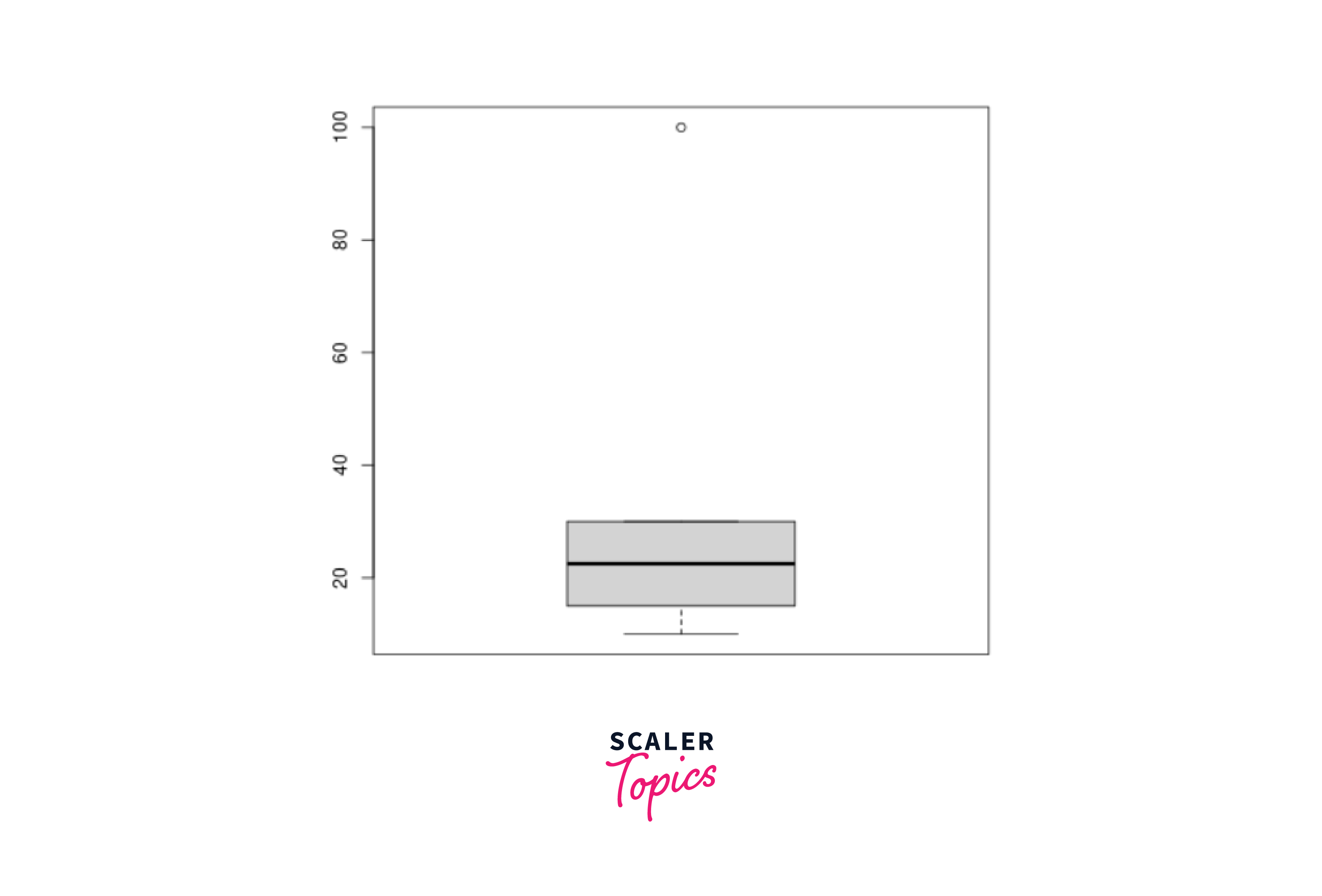
3. Dealing with Outliers:

Outliers are extreme values that deviate significantly from the overall data distribution. They can have a substantial impact on statistical analyses and model performance. Data cleaning involves identifying and handling outliers appropriately. Let's illustrate this with a vector containing outliers:

Output:

Data Transformation

In data wrangling, one of the fundamental distinctions we encounter is whether a dataset is presented in a wide or long format. The decision between wide and long datasets revolves around the choice of having more rows or more columns in the dataset. A dataset that prioritizes adding additional data about a single variable in its columns is termed a wide dataset because, as more columns are added, the dataset becomes wider. Conversely, a dataset that emphasizes including data about subjects in its rows is referred to as a long dataset.

Data wrangling in R often requires us to convert between wide and long datasets as per our analysis requirements. Data scientists who embrace the concept of tidy data typically favor long datasets over wide ones, as longer datasets are more amenable to manipulation in R.

Wide vs. Long:

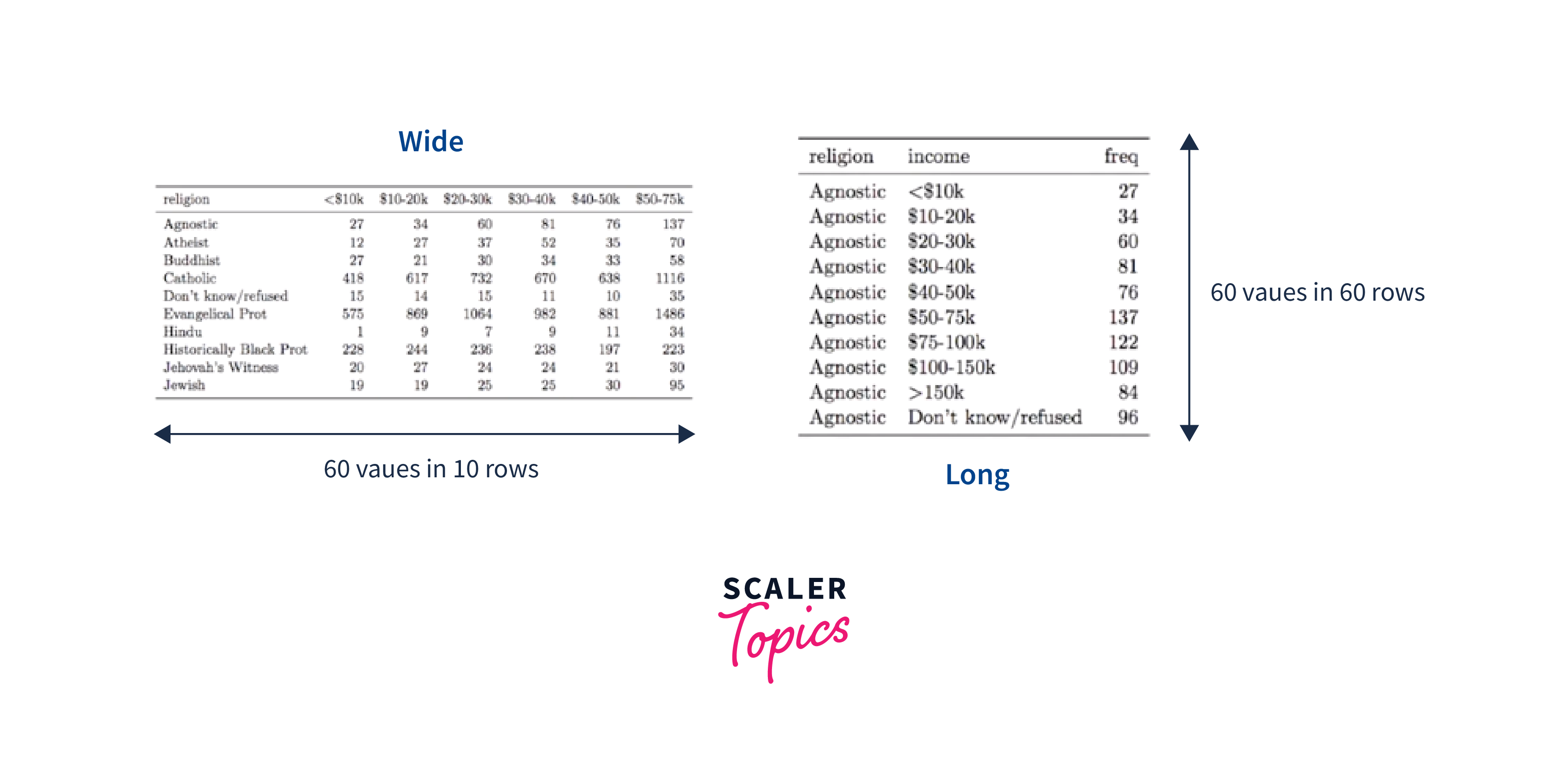
Consider the figure above, where the same dataset is represented in both wide and long formats. This dataset comprises religions and their income classifications. Understanding the distinction between long and wide datasets, let us now explore how to use R tools to convert between these two formats.

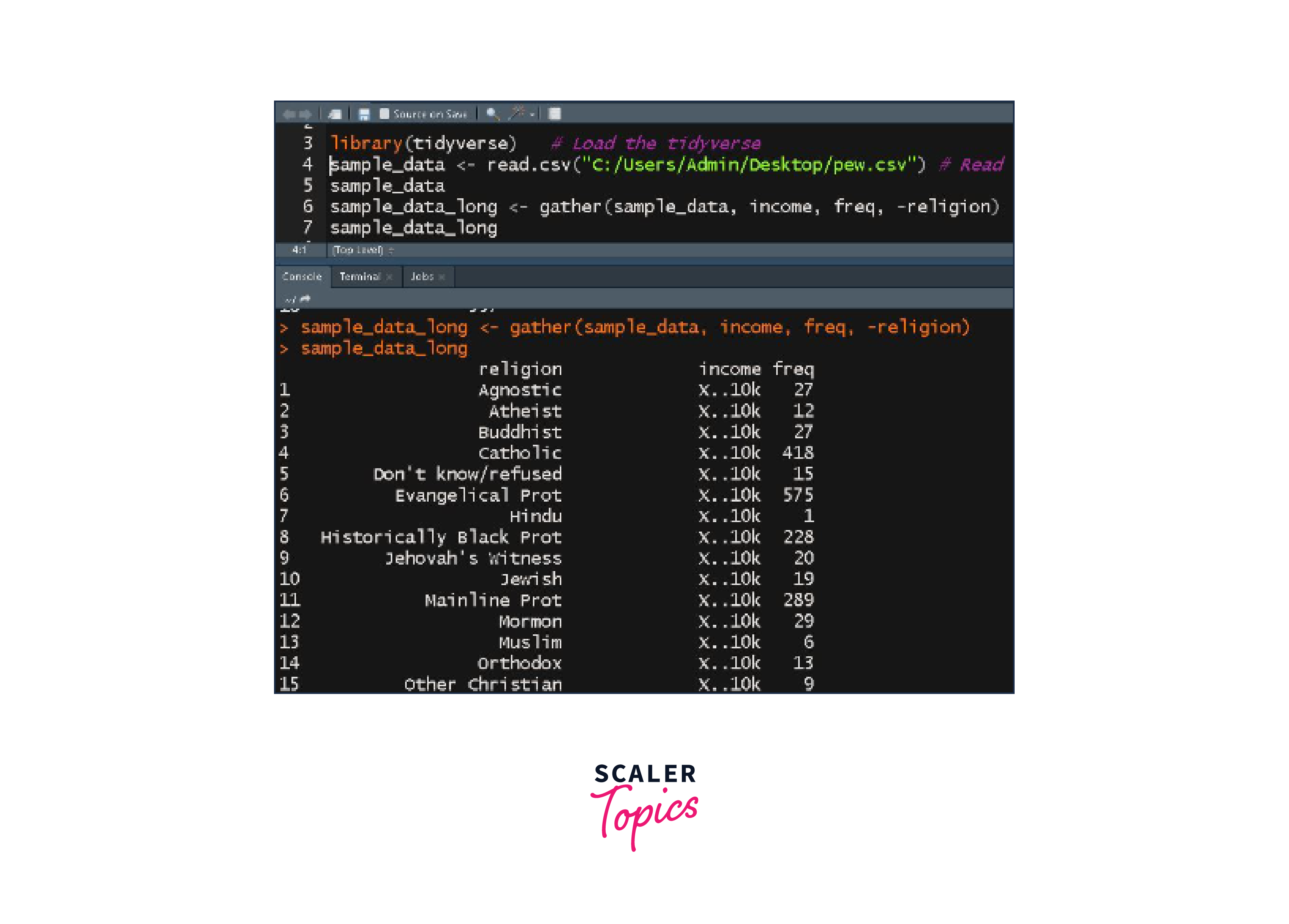
Conversion of Wide Dataset to Long:

To convert a wide dataset to a long one, we employ the gather() function from the 'tidyr' package. The gather function operates on the concept of keys and values. The keys represent the variable names, and the values represent the corresponding observations.

Syntax:

Parameters:

• data:
  The name of the data frame.
• key:
  The name to use for the key column in the long dataset.
• value:
  The name to apply for the value column in the long dataset.
• columns:
  A list of columns from the wide dataset to include or exclude from the gathering.

If you want to gather most of the columns, you can specify the columns to exclude by listing them with a minus sign (-) in front of their names.

Code Example - Converting Wide to Long:

Output:

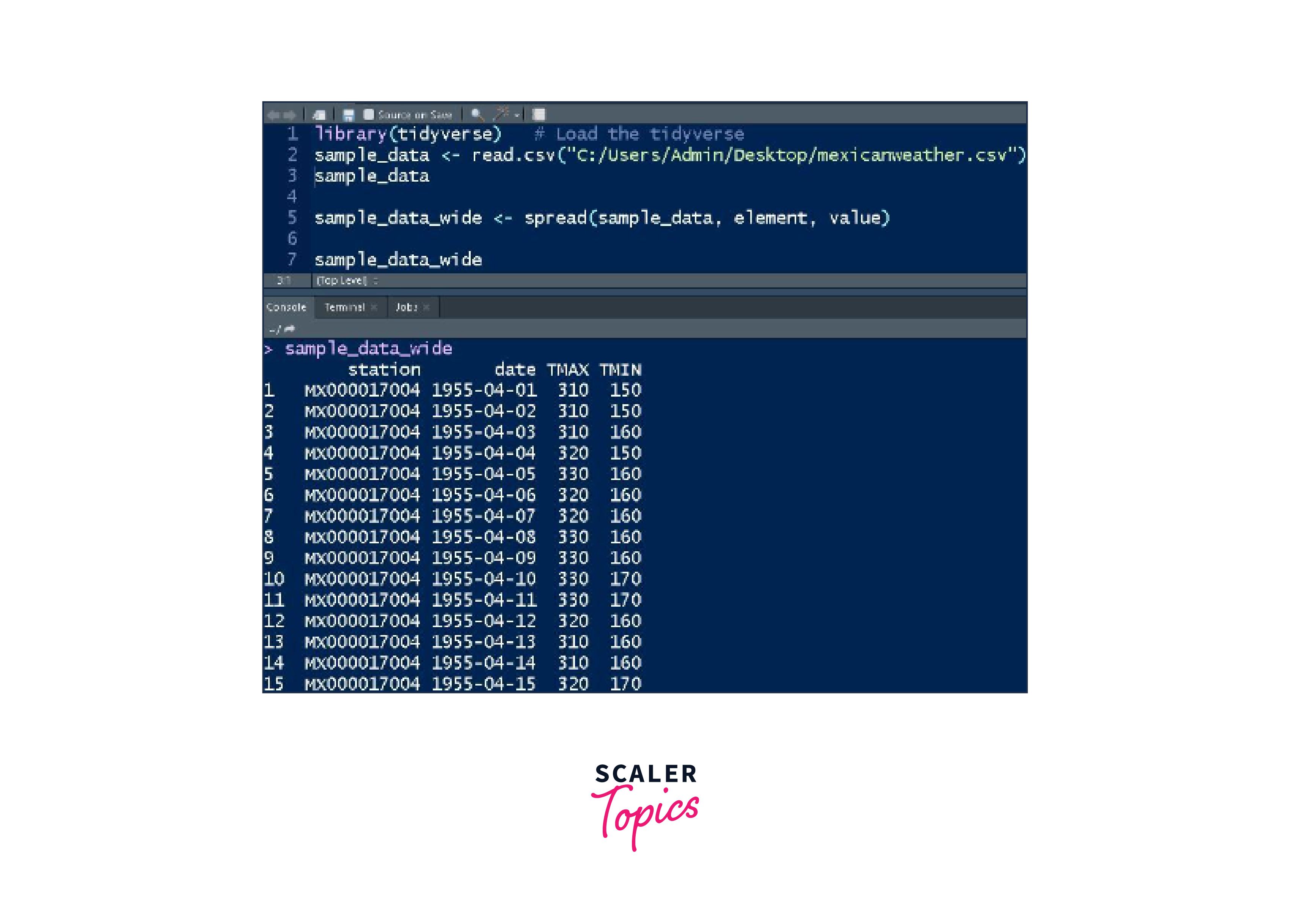
Conversion of Long Dataset to Wide:

Conversely, the spread() function is used to convert long datasets back into wider formats when needed.

Syntax:

Parameters:

• data:
  The name of the data frame.
• key:
  The name to use for the key column in the long dataset.
• value:
  The name to apply for the value column in the long dataset.

Code Example - Converting Long to Wide:

Output:

Data Visualization

Data visualization is an essential and integral step in the process of data wrangling in R. It plays a crucial role in gaining insights into the patterns and relationships present within the data. By utilizing packages like ggplot2 (part of the tidyverse suite of packages), data scientists can create insightful and visually appealing representations that not only facilitate better decision-making but also effectively communicate the findings to stakeholders.

Importance of Data Visualization:

Data visualization enables us to perceive complex data patterns, trends, and outliers that may not be immediately evident in raw data. Through visual representations like charts, graphs, and plots, we can identify correlations, distributions, and anomalies, which aid in making informed decisions based on data-driven insights.

Using ggplot2 for Data Visualization:

ggplot2 is a powerful and widely-used data visualization package in R. It follows the grammar of graphics, allowing users to construct and customize visualizations with a high level of flexibility and clarity. By specifying data mappings to visual attributes, such as color, shape, size, and position, ggplot2 helps create meaningful and informative plots effortlessly.

Code Example - Creating a Scatter Plot with ggplot2:

Let's illustrate the process of data visualization using ggplot2 with a simple scatter plot example. Assume we have a dataset named "data.csv" with two variables, "X" and "Y", representing the relationship between two quantitative variables.

Output :

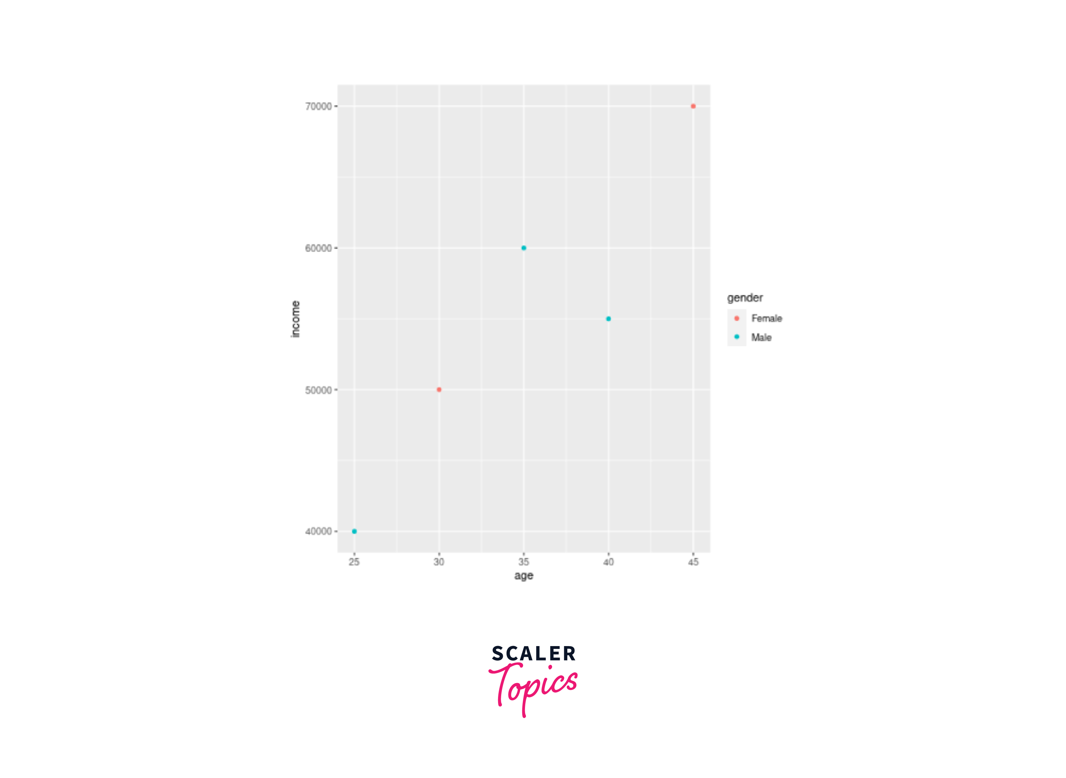
Explanation:

In the code example, we start by loading the required libraries, ggplot2 and readr. We then read the dataset "data.csv" into R using the read_csv() function from the readr package. After that, we create the scatter plot using the ggplot() function, where we specify the data source and the mapping of variables "X" and "Y" to the x-axis and y-axis, respectively. The geom_point() function adds the points to the plot, and the labs() function is used to provide the title and axis labels.

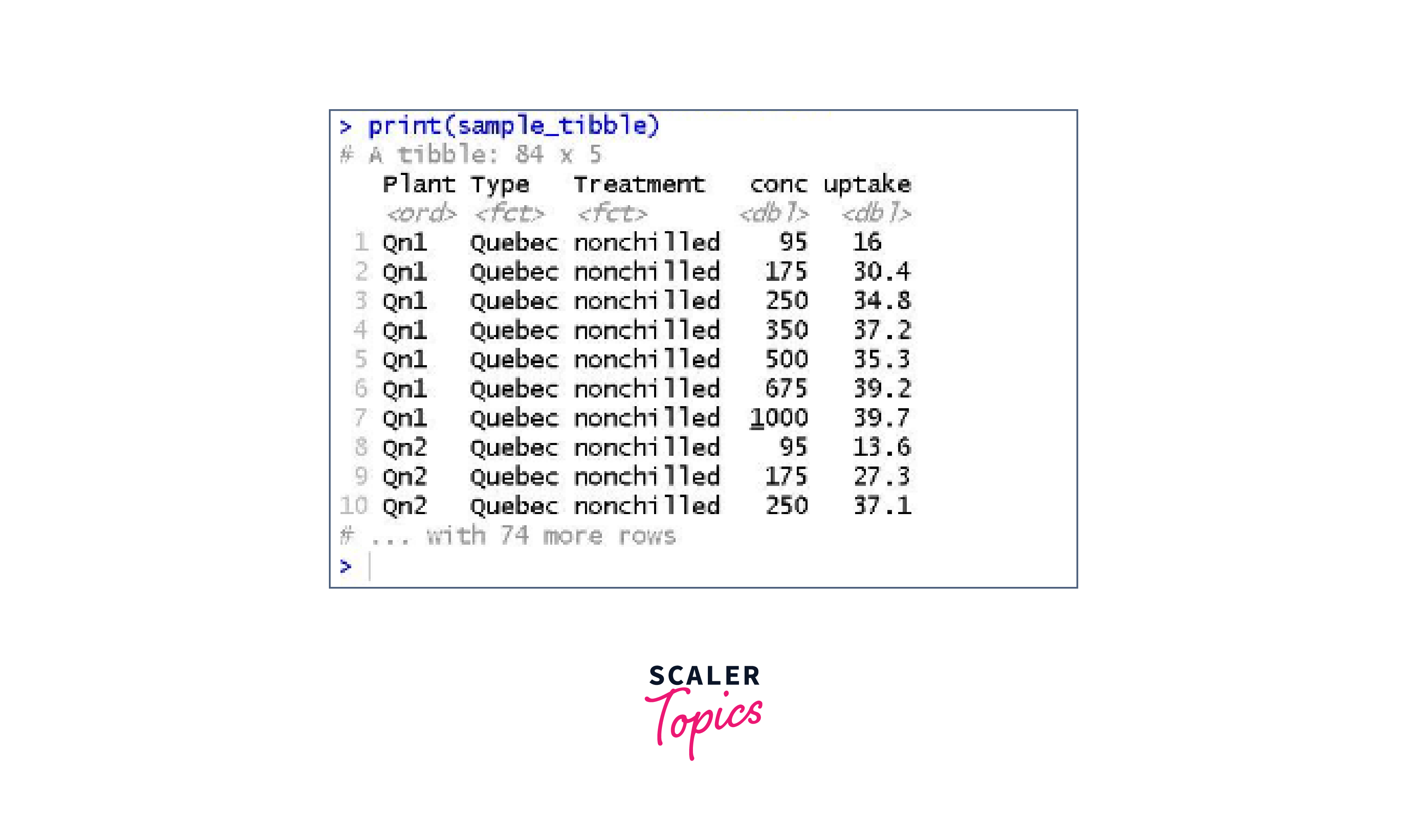
Working with Tibbles

Tibbles, the core data structure of the tidyverse, serve as a foundation for displaying and analyzing information in a tidy format. They represent an enhanced version of data frames, the most common data structures used to store datasets in R.

Advantages of Tibbles over Data Frames:

Tibbles offer several advantages over traditional data frames:

1. All Tidyverse packages fully support Tibbles.
2. Tibbles presents data in a cleaner format compared to data frames.
3. Unlike data frames, Tibbles avoid automatic conversion of character strings to factors, thus preventing the need for overriding settings

A. Different Ways to Create Tibbles

1. Using as_tibble():
   This function creates a Tibble from an existing data frame, matrix, or list.

   Code Example:

   Output:

   

2. Using tibble():
   This method allows creating a Tibble from scratch using name-value pairs.

   Code Example:

   Output:

3. Using Data Import Packages:
   The tidyverse's data import packages allow importing external data sources, such as databases or CSV files, and transforming them into Tibbles.

   Code Example:

B. Subsetting Tibbles

Data analysts often extract a single variable from a Tibble, which is known as subsetting. There are two ways to perform data subsetting:

1. Using the $ Operator:
Extracts a single variable from the Tibble in vector form.

Code Example:

Output:

2. Using the [[]] Operator:
Another method to access a single variable from the Tibble.

Code Example:

Output:

C. Filtering Tibbles

Filtering is a powerful technique to reduce the number of rows in a Tibble based on specified conditions.

Code Example:

Output:

Top Data Wrangling Functions

Data wrangling is an important stage in data analysis, and R provides the dplyr package to make this process simple and quick. We will look at some fundamental dplyr functions below:

1. select() - Selecting Columns in Your Data Set

To begin, let's focus on selecting specific columns from the dataset. For instance, we can select only the columns "mpg", "cyl", and "disp".

Output:

Alternatively, we can select all columns except the "hp" column.

Output:

We can also use the starts_with() function to select all columns that start with "d".

Output:

2. rename() - Renaming Columns

Next, we can rename columns to provide clearer descriptions. For example, we can rename the columns "mpg" to "Miles" and "cyl" to "NumberOfCylinder".

Output:

3. arrange() - Sorting Your Data Set

The arrange() function helps in sorting the data based on specified columns. We can sort by the "cyl" column.

Output:

We can also perform multiple-level sorting, such as first sorting by "mpg" in descending order and then by "cyl".

Output:

4. filter() - Filtering Rows in Your Data Set

The filter() function allows us to filter rows based on specific conditions. For instance, we can filter rows with the "cyl" 4.

Output:

We can apply multiple filters, such as filtering rows with the "cyl" (Number of cylinder) 6 and a Miles ("mpg") below the average.

Output:

Furthermore, we can filter rows with "cyl" (Number of cylinder) 6 and a Miles ("mpg") below the average, and where the gear is either 3 or 4.

Output:

5. mutate() - Generating New Columns in Your Data Set

The mutate() function helps in creating new columns based on existing ones. For example, we can create a column showing the rounded "disp" information.

Output:

6. summarize() - Creating Summary Calculations in Your Data Set

The summarize() function allows us to calculate summary statistics for the entire dataset. For example, we can calculate the mean and standard deviation for "mpg" and "disp".

Output:

7. group_by() - Grouping Your Data Set and Creating Summary Calculations

To create more meaningful summaries, we can use the group_by() function along with summarize(). For instance, let's group the data by "cyl" and then calculate summaries for "mpg" and "disp".

Output:

Grouping by more than one column is also possible. In the example below, we group by "cyl" and "gear".

Output: