Challenges in Training Deep Neural Networks

Introduction

Deep learning is a powerful and popular approach for building machine learning models, particularly for image and speech recognition, natural language processing, and more. However, training a deep learning model can be a complex and time-consuming process that involves a number of challenges and potential problems. In this discussion, we will explore some of the common problems that may arise during the training process and how to address them.

Challenges in Training Deep Neural Networks

Training deep learning models is a crucial part of applying this powerful technology to a wide range of tasks. However, training a model involves a lot of challenges from overfitting and underfitting to slow convergence and vanishing gradients; many factors can impact the performance and reliability of a deep learning model. Understanding these issues and how to mitigate them makes it possible to achieve better results and more robust models.

Network Compression

There is an increasing demand for computing power and storage. With that in mind, building higher efficiency models optimized for more performance with lesser computations is important. Here is where compression kicks in to give a better performance to computations ratio. A few methods for Network compression include,

• Parameter Pruning And Sharing - Reducing redundant parameters which do not affect the performance.
• Low-Rank Factorisation - Matrix decomposition to obtain informative parameters of CNN.
• Compact Convolutional Filters - A special Kernel with reduced parameters to save storage and computation space.
• Knowledge Distillation - Train a compact model to reproduce a complex one.

Pruning

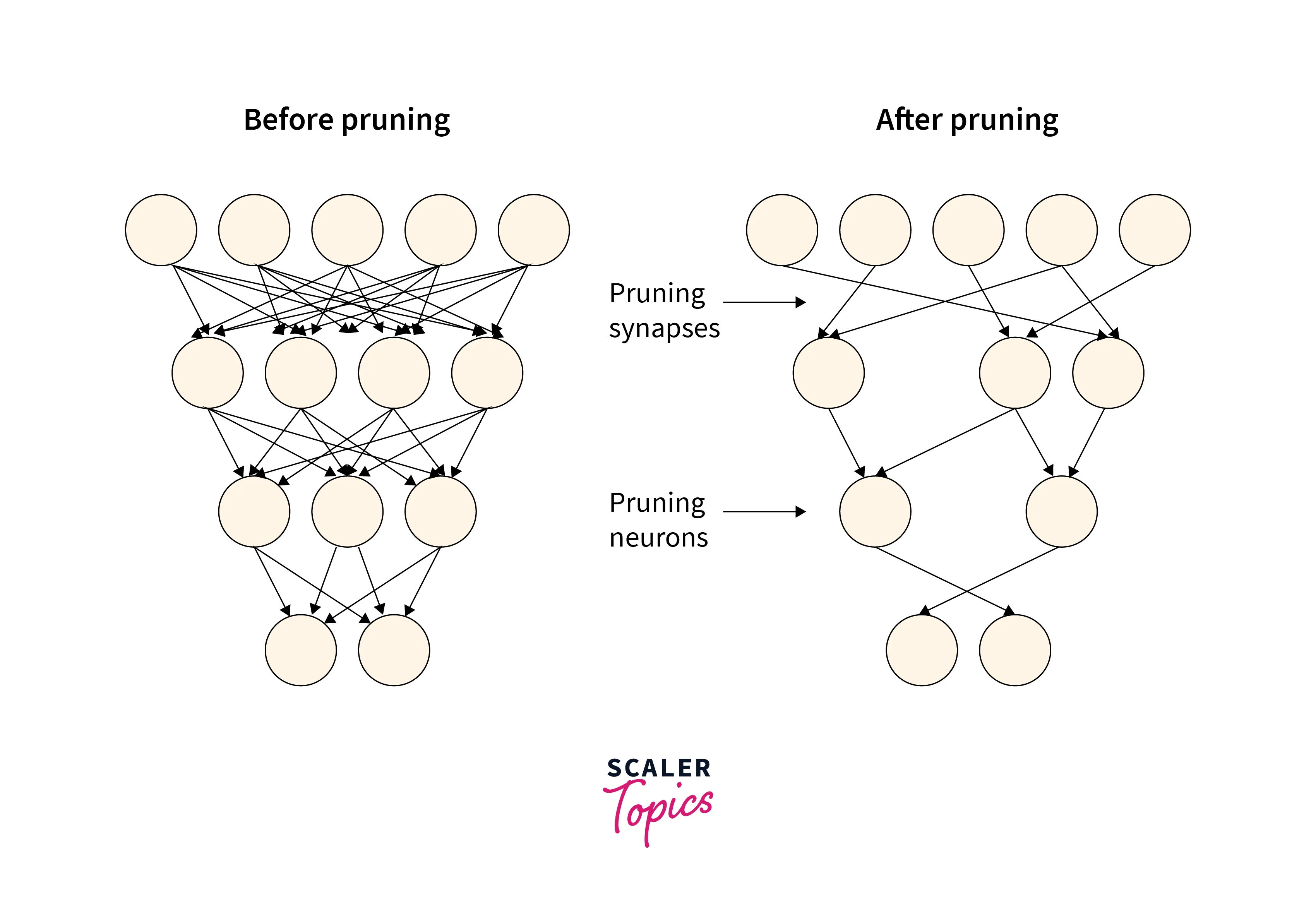
Pruning is the method of reducing the number of parameters by removing redundant or insensitive neurons. There are two methods to prune

• Pruning by weights involves removing individual weights from the network that are found to be unnecessary or redundant. This can be done using a variety of methods, such as setting small weights to zero, using magnitude-based pruning, or using functional pruning. Pruning by weights can help to reduce the size of the network and improve its efficiency, but it can also reduce the capacity of the network and may lead to a loss of performance. This keeps the architecture of the model the same.

• Pruning by neurons involves removing entire neurons or groups of neurons from the network that are found to be unnecessary or redundant. This can be done using a variety of methods, such as using importance scores to identify and remove less important neurons or using evolutionary algorithms to evolve smaller networks.

Reduce the Scope of Data Values

In a Neural Network, the weights, biases, and other parameters are initialized to take up 32-bit of information. 32-bit variables add precision to the model by adding more values after the decimal point. But in practical applications, reducing the precision from 32-bit to 16-bit floating point does not change the model's output.

Suppose we have a simple neural network with one input, one hidden layer with two neurons, and one output. The weights and biases of the network are initialized using 32-bit floating point values. The network is trained on a dataset and can achieve a certain level of accuracy.

Now, we want to improve the efficiency of the network by reducing the precision of the weights and biases from 32-bit to 16-bit floating point values. We can do this by simply casting the 32-bit values to 16-bit values and using them to initialize the network.

During training, we find that the network can achieve the same level of accuracy with the reduced precision weights and biases as it did with the full precision weights and biases. This means that we were able to improve the efficiency of the network without sacrificing performance.

Overall, reducing the precision of the weights and biases in a neural network can be a useful technique for improving efficiency without sacrificing performance, but it is important to consider the trade-offs involved carefully and to carefully test the impact of reducing precision on the final model.

Bilinear CNN

A Bi-Linear CNN architecture solves the problem of image recognition in fine-grained image datasets.

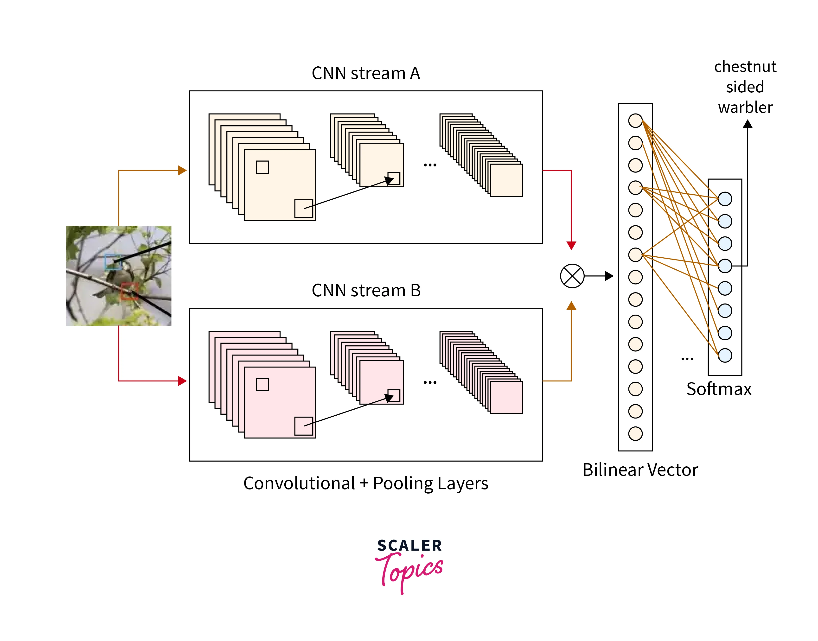
A Bilinear CNN contains 2(or sometimes more) CNN feature extractors, which identify different features. The different feature extractors are combined as a Bilinear Vector to find the relationship between the different features. This is passed through a classifier to obtain the results. For example, If the task was to recognize a bird, One feature extractor would identify the tail, while the other would identify the beak. These two will then come together to infer if the image presented to it is a bird at the bilinear vector.

Vanishing/Exploding Gradients Problems

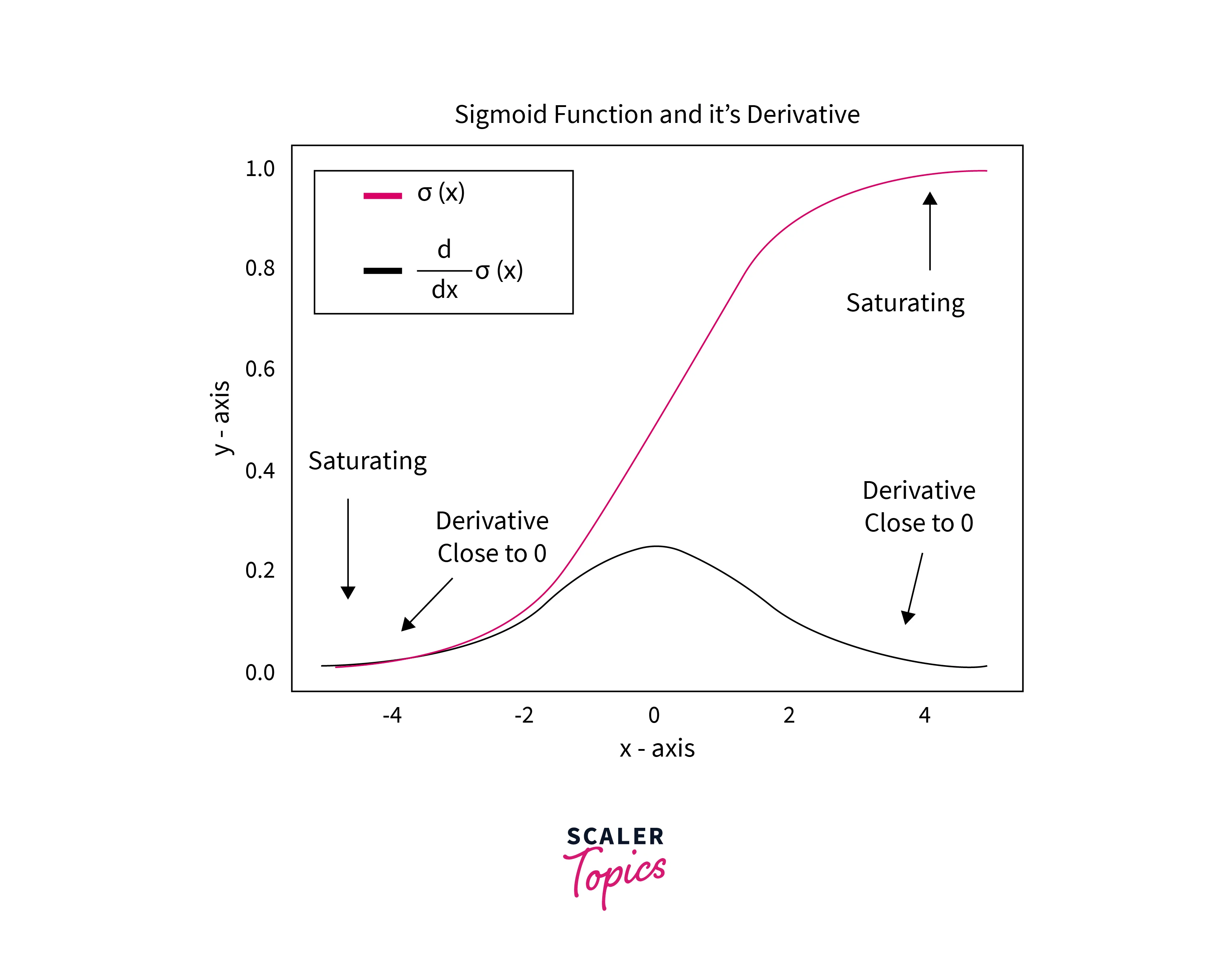
The vanishing/exploding gradient problem occurs during backpropagation. In Backpropagation, we try to find the gradients of the loss function concerning the weights. During the backpropagation algorithm, we will be required to multiply values numerous times depending on the number of layers. If the value of weights is small(lesser than 1), the backpropagation method will make the value of the weights smaller and smaller until it becomes almost zero. This is the vanishing gradient problem.

Exploding gradient problem is similar but with very large weight values. If the weights become too big, the backpropagation algorithm makes them bigger and bigger, making it difficult, sometimes impossible, to compute and train.

The reason for the Vanishing gradient is the Tanh and Sigmoid Activation function. Tanh activation function contains values between -1 and 1. At the same time, the Sigmoid activation function contains values between 0 and 1. These two activation functions map any value between small ranges, thus creating the vanishing gradient problem.

Non-saturating Activation Function

One problem that can occur with activation functions is non-saturation, which refers to the inability of the activation function to saturate, or reach its maximum output value. This can lead to several issues, such as the inability of the network to learn, poor generalization, and slow convergence.

There are several common activation functions that can suffer from non-saturation, including the linear activation function and the sigmoid activation function. These activation functions can saturate when the input to the activation function is very large or very small, but they may not saturate for intermediate input values. This can make it difficult for the network to learn and can lead to slow convergence.

Suppose we have a simple neural network with one input, one hidden layer with two neurons, and one output. The hidden layer uses the sigmoid activation function, which is defined as:

Where x is the input to the activation function.

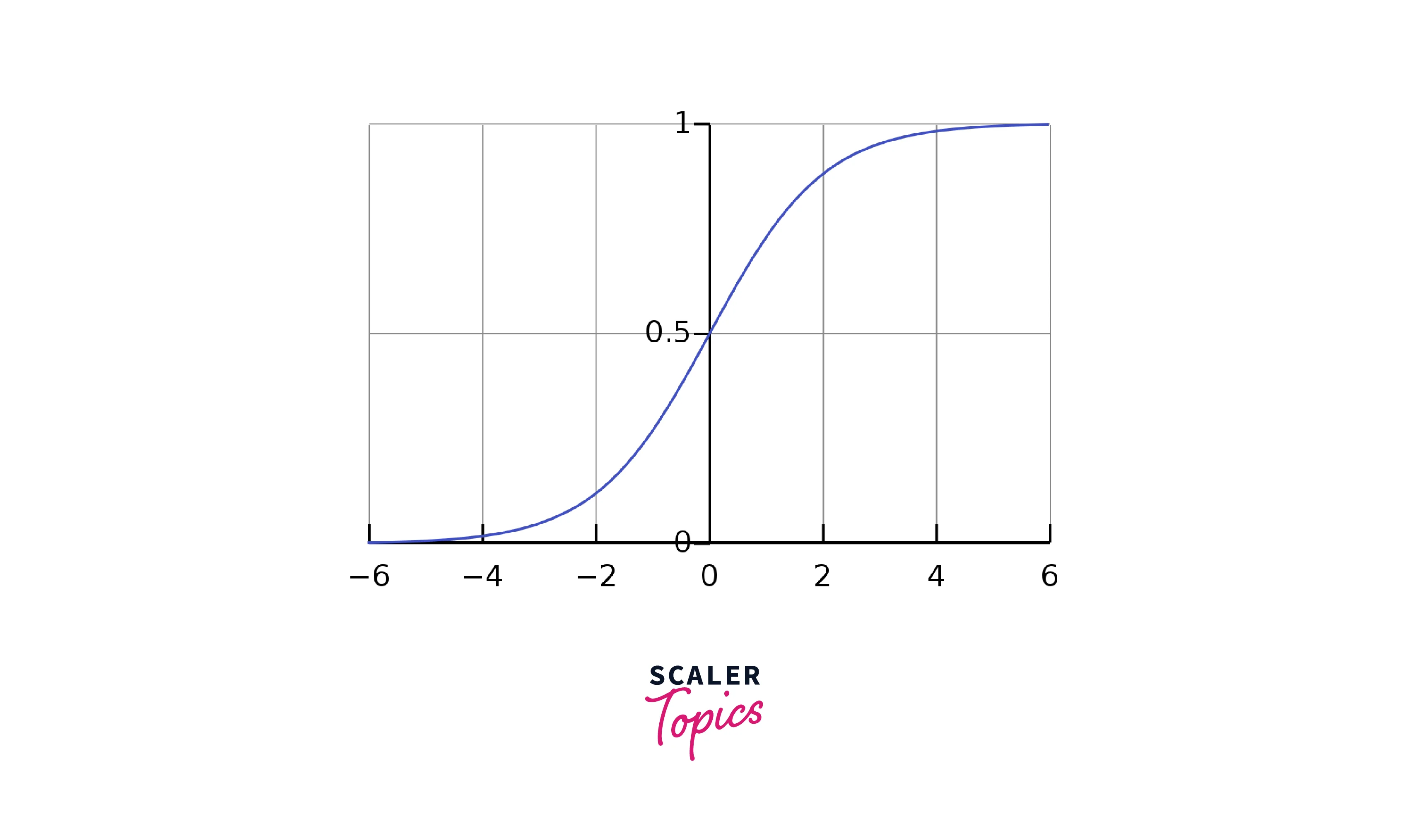
The input to the first hidden neuron is -5, and the input to the second hidden neuron is 5. The output of the first hidden neuron will be very close to 0 (since $e^{(-5)}$ is very small), and the output of the second hidden neuron will be very close to 1 (since $e^{(5)}$ is very large).

This means that the sigmoid activation function has saturated for both of these input values, and the neural network will not be able to learn effectively because the gradient of the activation function will be very close to 0 for these inputs. This can lead to slow convergence and poor generalization.

Using an activation function that is more effective at saturating, such as the ReLU, can help to avoid this issue and improve the performance of the neural network.

Batch Normalization

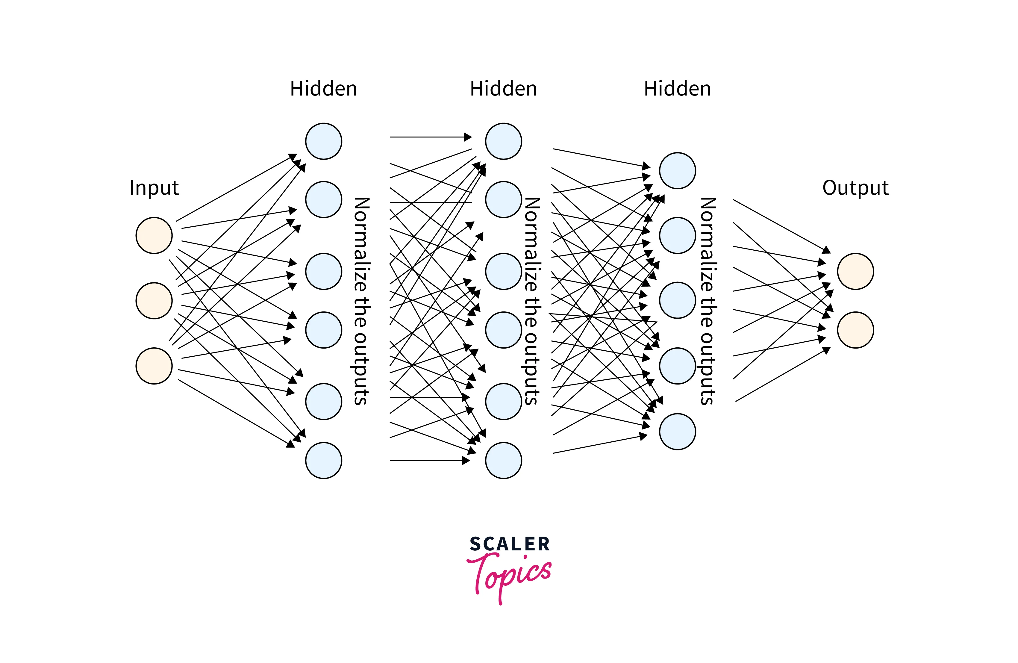
Batch Normalization is a method of Normalizing the data after every activation function. Normalizing means bringing every value of data within the same range. Keeping the range of data small equals faster training time. It also helps with the problem of internal co-variate shift, which means during backpropagation, each neuron tries to minimize its loss concerning the result obtained in the previous layer. The result of the previous layer might change in the next iteration, and this problem gets amplified with deeper layers. So it feels like chasing a moving target. This problem is referred to as the internal covariate shift. Batch Normalization helps minimize this problem as well.

Gradient Clipping

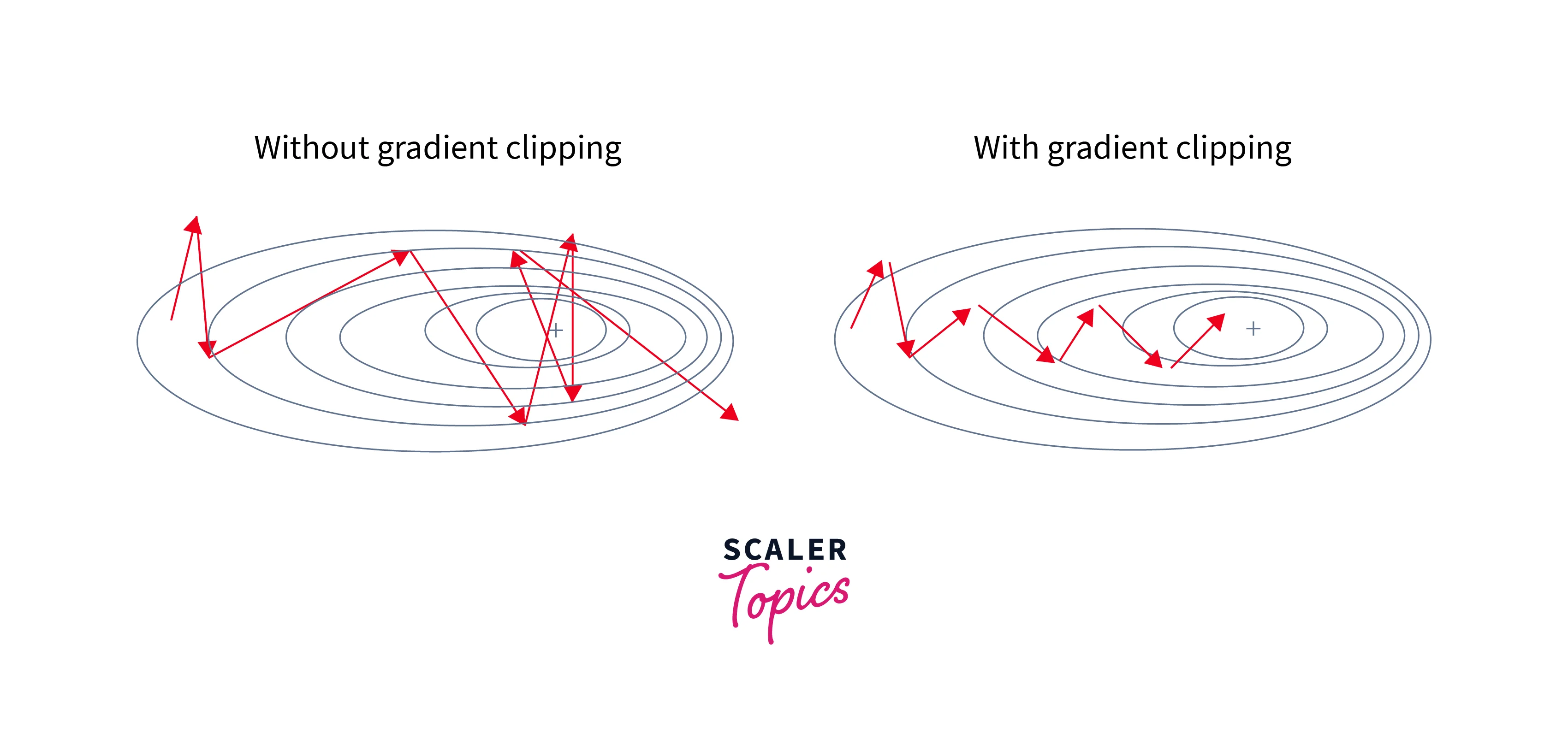
Gradient clipping is a very useful technique to overcome the exploding gradient problem. In this method, the gradients are limited to a threshold and made sure it doesn't exceed the value. Keeping the gradients in check helps to escape the exploding gradient problem. It is especially useful in LSTMs where Exploding Gradient might occur due to the Tanh and Sigmoid Activation functions. There are two methods to implement gradient clipping.

• Clipping by value: The gradients are given a min and max value. The max or min bound value is taken if the gradient exceeds the bounds.
• Norm clipping: All the gradients are clipped by a certain value to always stay below the norm value.

Additional Resources

1. Difference Between Machine Learning and Deep Learning