Density Plot in R
Overview
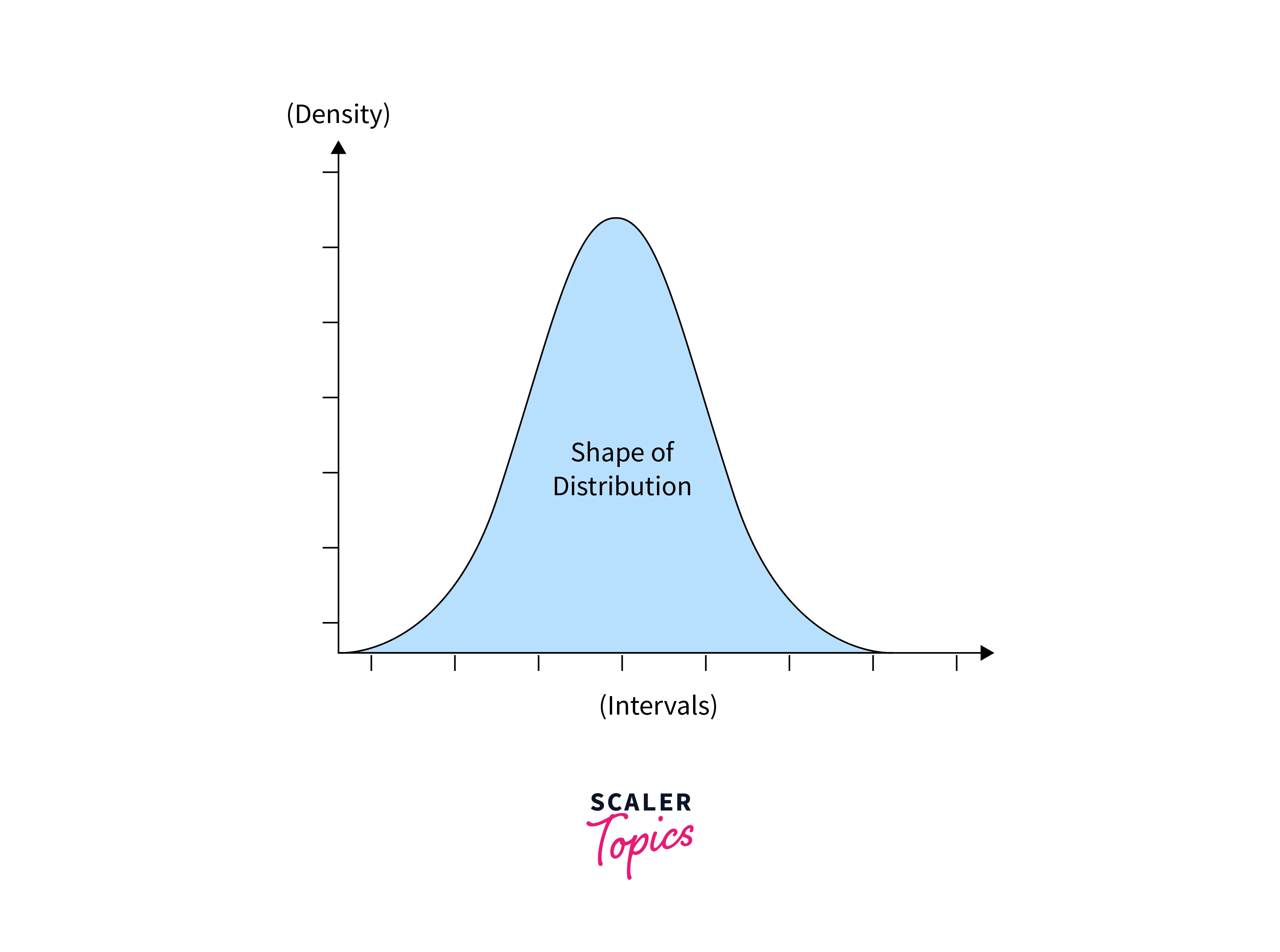
A Density Plot in R is a data visualization technique used to display the distribution of a continuous variable. It provides a smooth representation of the data's probability density, offering insights into its shape and spread. By plotting a smoothed curve, often resembling a histogram, Density Plots highlight areas of high and low data concentration. They are particularly useful for identifying patterns and trends in data, aiding in exploratory data analysis and statistical inference. Density Plots provide a visual summary of data distribution, making them a valuable tool for understanding the underlying characteristics of a dataset in a compact and informative manner.
What are Density Plots?
Density Plots in R are a type of data visualization that provides a smoothed representation of the distribution of a continuous variable. They offer insights into the underlying probability density function of the data, highlighting areas of higher and lower data concentration. Density Plots are particularly useful for understanding the shape, spread, and central tendencies of a dataset.
In a Density Plot, data points are converted into a continuous smoothed curve, often resembling a histogram. This curve represents the estimated probability density of the variable at different values along its range. Unlike histograms that use discrete bins, Density Plots offer a continuous view of the distribution, making them less sensitive to the choice of bin size and revealing subtle patterns that might be missed with discrete representations.
Density Plots can be created in R using various functions, such as geom_density() in the ggplot2 package or the base R function density(). They can be customized with different line styles, colors, and bandwidths to control the level of smoothing. Additionally, Density Plots can be overlaid with other plots to facilitate comparisons between multiple distributions.
How to Create a Basic Density Plot in R ?
Plotting a Simple Density Plot
To create a simple Density Plot in R, you can use the density() function to estimate the probability density of a continuous variable and then use the plot() function to visualize the density curve. Here's a step-by-step example of how to plot a simple Density Plot using randomly generated data:
In this example:
- We generate random data using rnorm() to simulate a dataset with 1000 normally distributed values.
- The density() function estimates the probability density of the data.
- The plot() function is used to create the Density Plot. We pass the density_data object, set the plot title (main), and label the x-axis (xlab) and y-axis (ylab).
- When you run this code, it will display a simple Density Plot showing the estimated density curve of the randomly generated data.
Customizing Plot Colors and Styles
Customizing plot colors and styles in R allows you to enhance the visual appeal and effectiveness of your visualizations. You can use various functions and parameters to modify colors, line styles, markers, and more. Here's a guide on how to customize plot colors and styles:
- Changing Line Colors and Styles:
You can specify line colors and styles using the col and lty parameters within plot functions. For example:
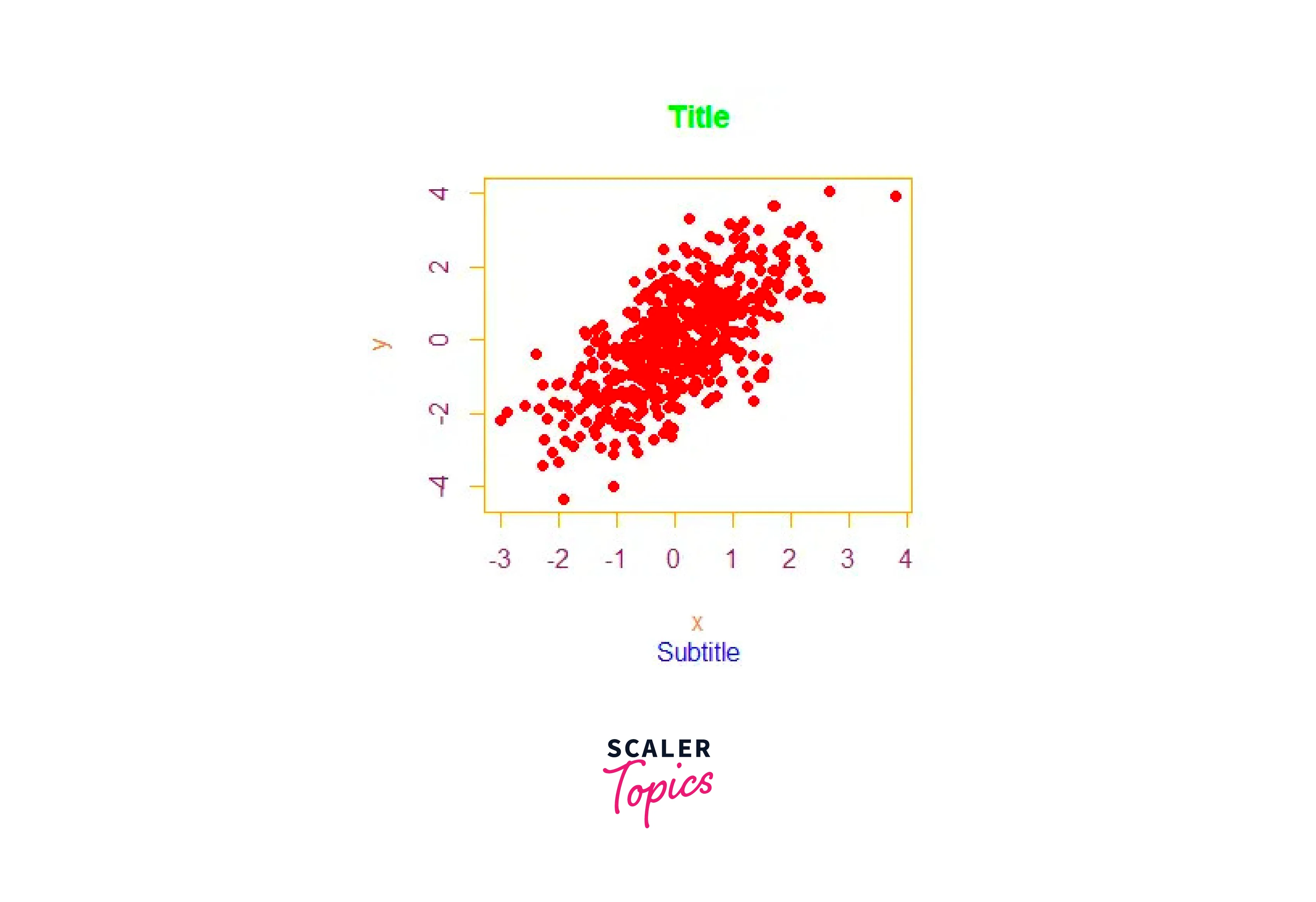
- Adding Points and Customizing Markers:
To add points to your plot and customize their appearance, you can use the points() function. You can modify parameters such as pch (marker type), col (marker color), and cex (marker size). For instance:
- Customizing Axes and Labels:
You can customize axis labels, titles, and other text elements using functions like axis(), title(), and text(). For example:
- Using Color Palettes:
R offers various color palettes that can be applied to your plots. The palette() function sets the default color palette, and the col parameter in plot functions can be used to apply specific palettes.
- Creating Legends:
Legends help identify elements in your plot. You can add legends using the legend() function, specifying positions, colors, and labels.
- Combining Multiple Plots:
You can create complex plots by combining multiple visualizations using functions like par() and layout(). This allows you to customize each component separately.
Adding Labels and Titles
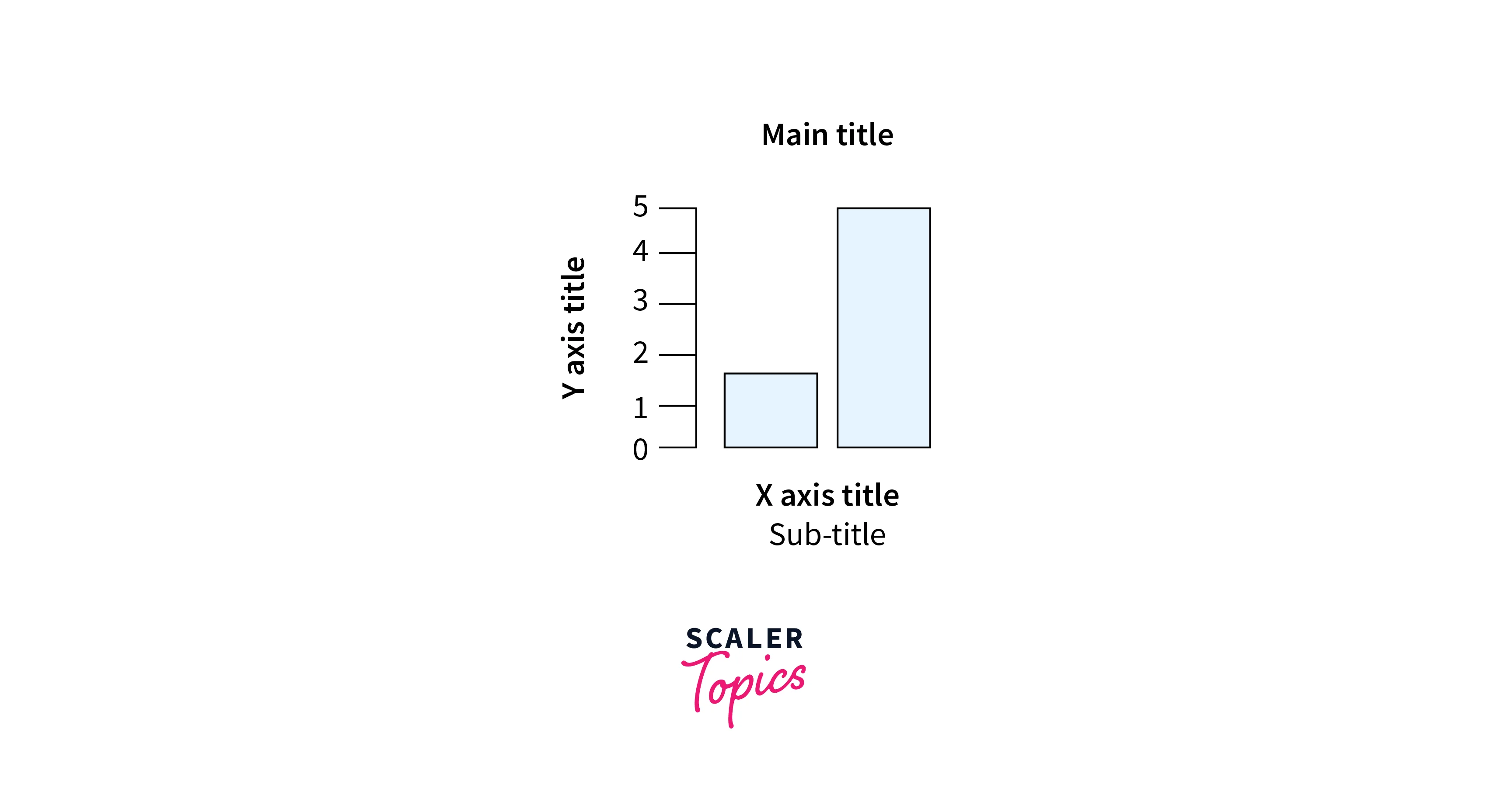
Adding labels and titles to your plots in R is essential for providing context and enhancing the interpretability of your visualizations. You can use functions like title(), xlab(), ylab(), and main() to add labels and titles to different aspects of your plots. Here's how to do it:
- Adding Main Title:
The main() function is used to add a main title to your plot. This title provides an overall description or summary of the plot's content.
- Adding Axis Labels:
The xlab() and ylab() functions allow you to label the x and y axes, respectively.
- Adding Text Annotations:
You can use the text() function to add annotations, labels, or notes at specific coordinates within the plot.
- Creating Legends:
Legends help identify different elements or groups in your plot. You can use the legend() function to add a legend at a specified position.
- Customizing Font and Style:
You can customize the font size, style, and color of labels and titles using the font, cex, and col parameters.
- Multiline Titles:
If you want to have multiline titles, you can use the "\n" character to indicate line breaks.
Adding labels and titles is a crucial step in enhancing the clarity and interpretation of your plots. By providing context and information, you make your visualizations more accessible and meaningful to your audience. Experiment with different label placements, styles, and formatting to find the best way to convey your data's insights effectively.
Kernel Density Plots
Introduction
Kernel density plots and density plots are related visualizations used to display the distribution of data in R, but they are not the same. Let's explore the differences between them:
Density Plot:
A density plot is a graphical representation of the distribution of a continuous variable. It provides an estimate of the probability density function of the data. In a density plot, the y-axis represents the density (or frequency), while the x-axis represents the values of the variable being analyzed. The plot is created by smoothing the data points to generate a continuous curve.
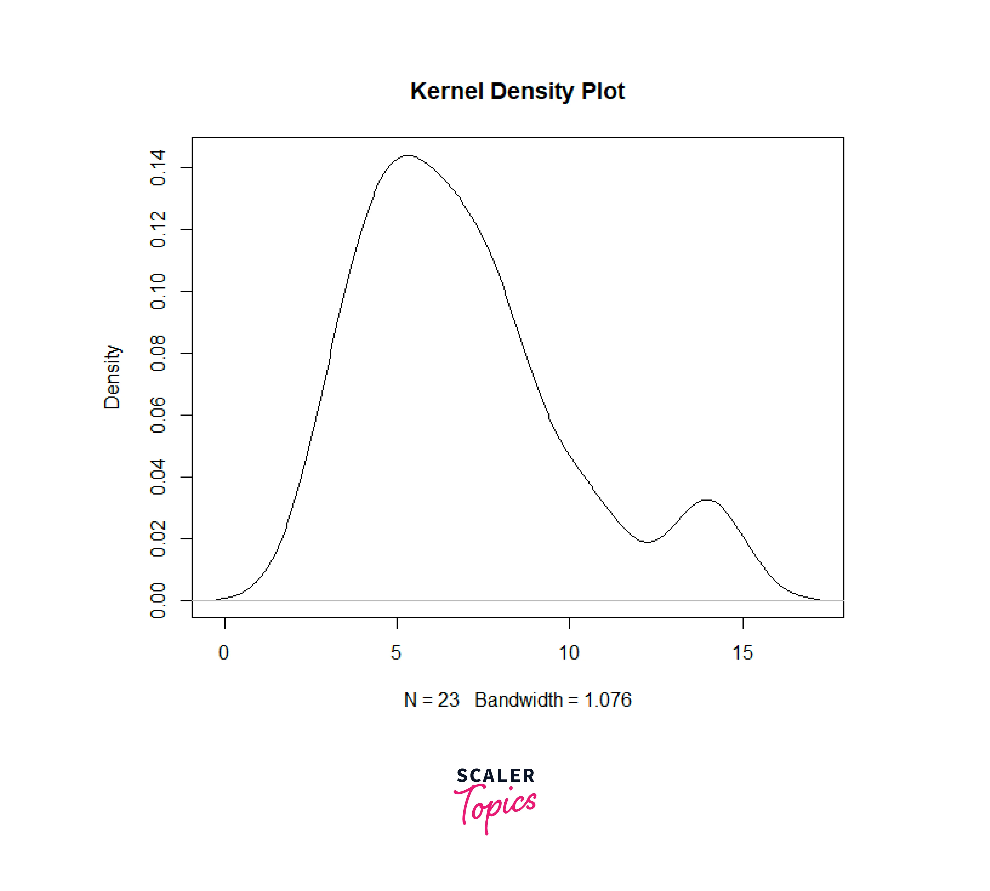
Kernel Density Plot:
A kernel density plot is a type of density plot that uses kernel smoothing to estimate the probability density function of the data. It is a more flexible and continuous version of the histogram. In kernel density plots, each data point contributes a small Gaussian curve (kernel) at its location, and these individual curves are summed to create the overall smoothed curve.
Key Differences:
| Density Plot | Kernel Density Plot | |
|---|---|---|
| Smoothing and Continuity | - Density plots can have gaps between the bins, resulting in a less continuous appearance. | - Kernel density plots are more continuous and provide a smoother representation of the distribution due to the use of kernel smoothing. |
| Flexibility | - Density plots might not handle irregularly spaced data points as effectively as kernel density plots. | - Kernel density plots are more flexible in handling irregular data and provide a more accurate representation of the distribution. |
| Kernel Selection | - Density plots don't involve the concept of kernel selection, as they use a predefined approach. | - Kernel density plots allow the choice of kernel function (e.g., Gaussian, Epanechnikov) that affects the smoothing process. |
| Choice of Parameters | - Density plots often require fewer tuning parameters. | - Kernel density plots might involve parameter tuning for kernel bandwidth, affecting the smoothness of the curve. |
| Interpretability | - Density plots can be easier to interpret due to the presence of distinct bins. | - Kernel density plots might require a better understanding of kernel smoothing and Gaussian functions for interpretation. |
How to Create Kernel Density Plots
Kernel Density Plots (KDPs) are versatile and insightful visualization tools in R for understanding the distribution of continuous variables. They offer different approaches to effectively visualize data density and uncover underlying patterns. In this detailed exploration, we will delve into three distinct approaches to creating Kernel Density Plots in R: One Kernel Density Plot, Filled Kernel Density Plot, and Multiple Kernel Density Plots.
- Approach 1: One Kernel Density Plot
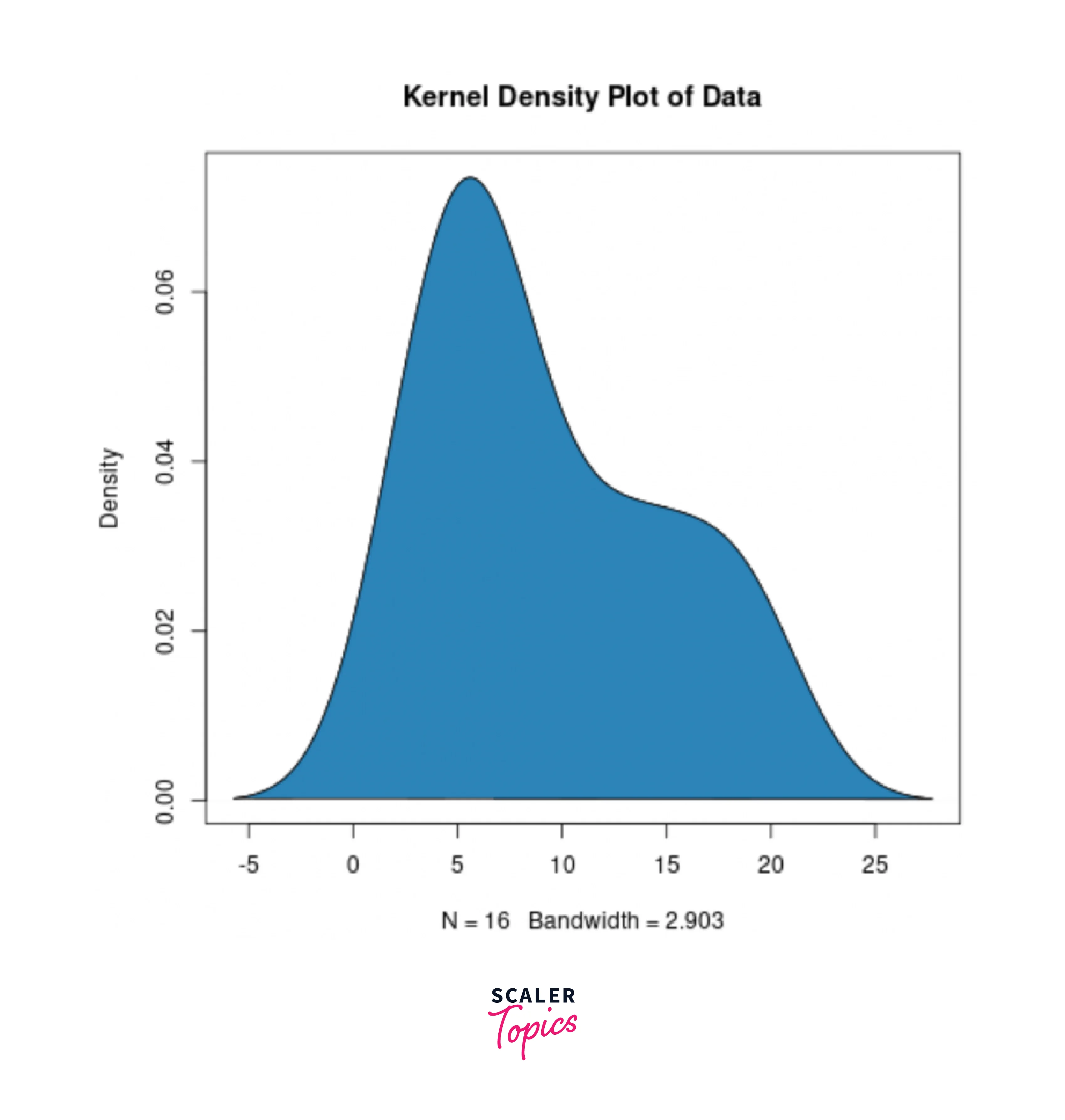
The first approach involves creating a single Kernel Density Plot to visualize the distribution of a single continuous variable. This provides an overview of the data's density, helping us identify modes, skewness, and concentration. To create a single Kernel Density Plot in R, we use the density() function to estimate the smooth density curve and then use the plot() function to visualize it.
This approach provides a concise representation of the data's distribution and is particularly useful for understanding the overall shape and concentration of the variable.
- Approach 2: Filled Kernel Density Plot
The second approach enhances the clarity of the Kernel Density Plot by filling the area under the curve with color, creating a Filled Kernel Density Plot. This not only emphasizes the distribution but also facilitates visual comparison between different parts of the curve. To create a Filled Kernel Density Plot, we use the polygon() function to fill the area under the curve.
The Filled Kernel Density Plot offers a visually appealing representation of the data distribution, allowing us to observe areas of high and low density more distinctly.
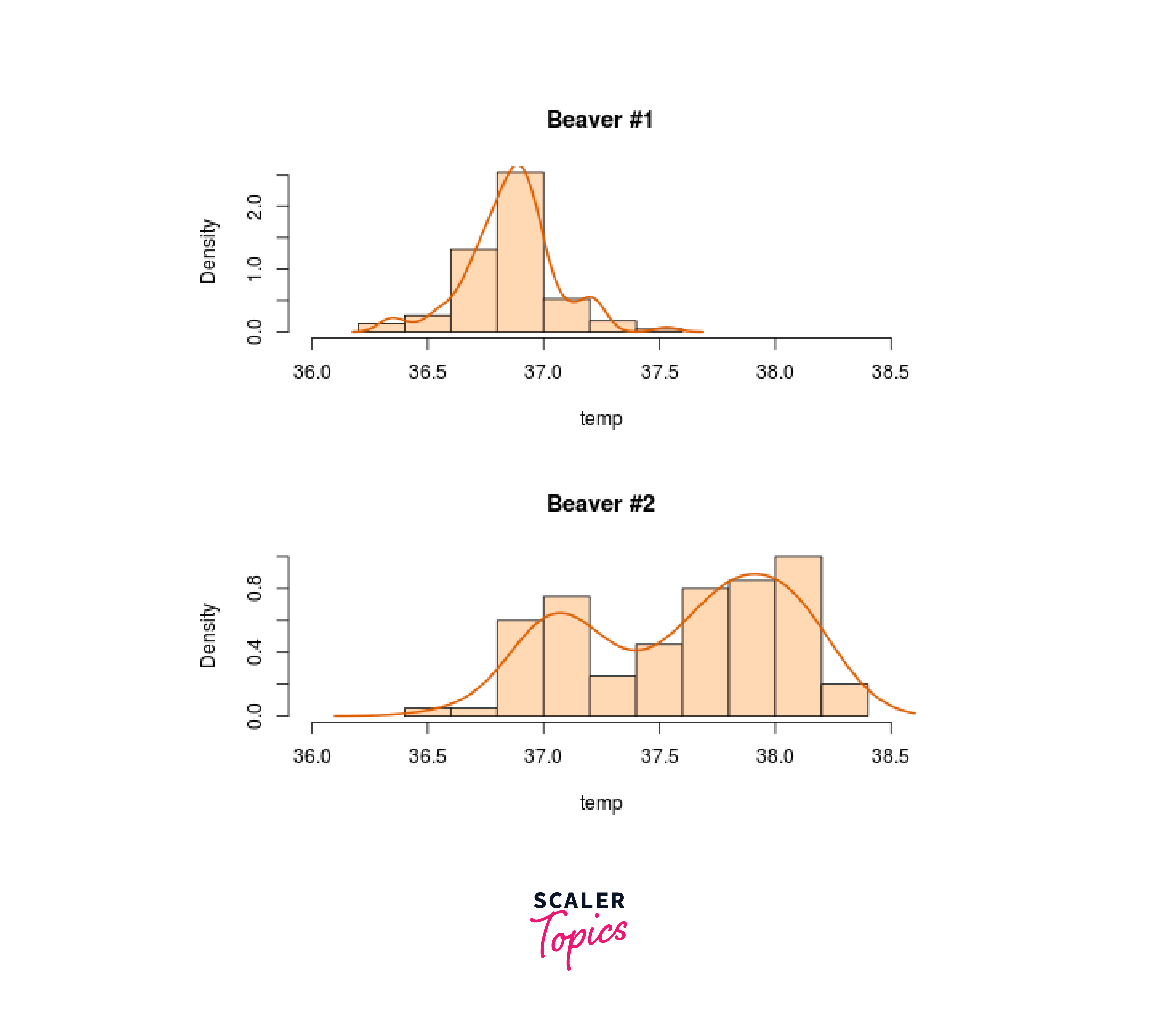
- Approach 3: Multiple Kernel Density Plots
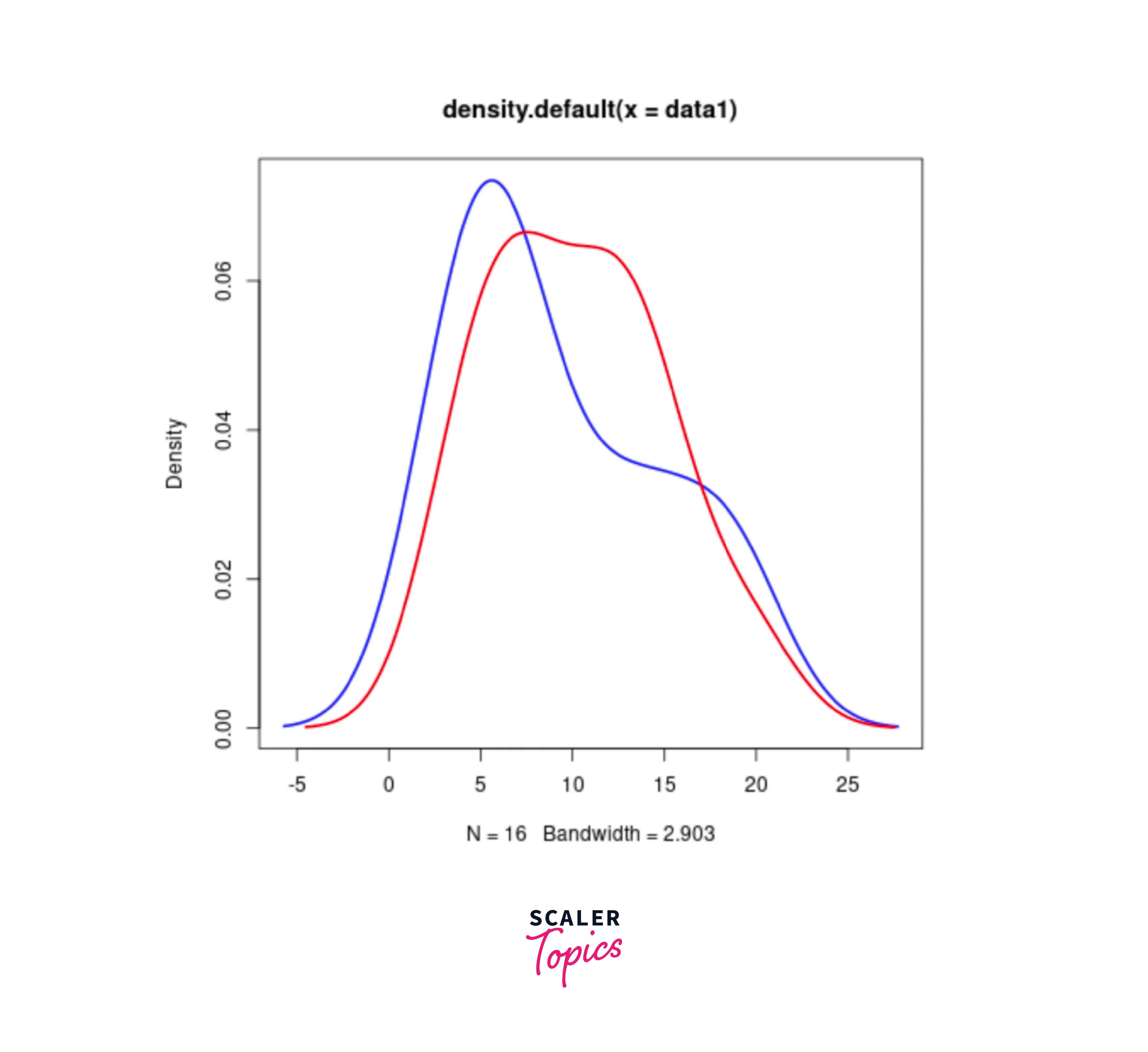
The third approach involves creating Multiple Kernel Density Plots to compare the distributions of multiple continuous variables or groups. This approach helps us identify differences and similarities between distributions, making it valuable for comparative analysis. To create Multiple Kernel Density Plots, we overlay multiple density curves on a single graph using the lines() function.
The Multiple Kernel Density Plots offer a clear comparison between the distributions of two groups, highlighting any differences in their density patterns.
Density Plot with ggplot2 Library
Density plots, a popular visualization technique for displaying data distribution, can be easily generated using the ggplot2 library in R. ggplot2 offers a powerful and flexible grammar of graphics that allows you to create sophisticated visualizations with ease. In this detailed guide, we'll walk through the process of creating density plots using ggplot2, from data preparation to customization.
- Step 1: Install and Load the ggplot2 Library
Before you start, make sure you have the ggplot2 library installed. If not, you can install it using:Then load the library:
- Step 2: Prepare Your Data
For demonstration purposes, let's assume you have a dataset named data with a continuous variable named value. Replace this with your actual data and variable. - Step 3: Create the Density Plot
To create a density plot using ggplot2, follow these steps:This code snippet creates a simple density plot using the geom_density() function. The aes(x = value) mapping specifies that the value variable should be plotted on the x-axis.
- Step 4: Customize the Plot
ggplot2 provides a wide range of customization options to tailor your density plot:- Adjusting Bandwidth:
You can customize the bandwidth of the density estimation using the adjust parameter within geom_density(). For example: - Color and Fill:
You can change the color of the density line or the fill color using the color and fill parameters. For example: - Adding Titles and Labels:
You can add titles and axis labels using the labs() function: - Themes:
You can apply different themes to your plot to change its appearance. For example:
- Adjusting Bandwidth:
- Step 5: Multiple Density Plots and Grouping
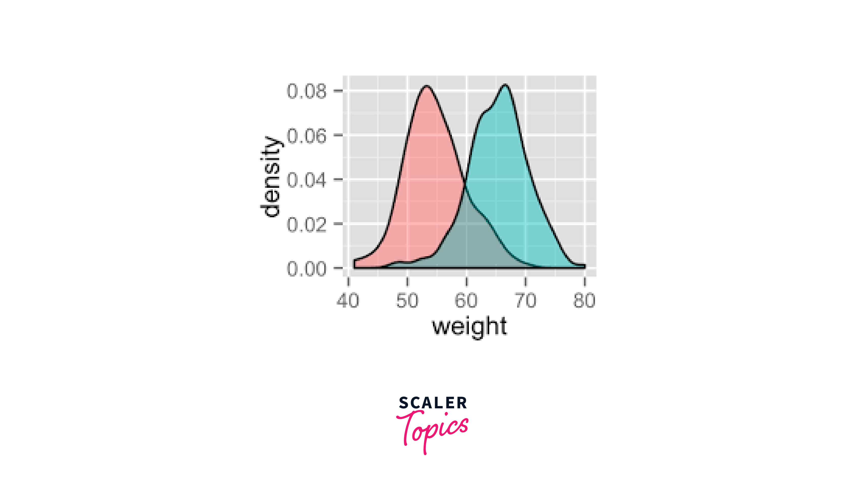
You can create multiple density plots for different groups using facets or grouping. Here's an example of grouping by a categorical variable named group:
In this example, the fill aesthetic fills the density curves by group, and the alpha parameter controls the transparency of the fill colors.
Customising Density Plots in R
Change Density Plot Line Types and Colors
Customizing the line types and colors of a density plot in R allows you to emphasize different aspects of the data distribution and enhance the visual appeal of the plot. You can achieve this by modifying parameters within the geom_density() function of the ggplot2 library. In this guide, we'll demonstrate how to change the line types and colors of a density plot.
Assuming you have loaded the necessary libraries and prepared your data, follow these steps to change the density plot line types and colors:
-
Step 1: Create a Basic Density Plot
Start by creating a basic density plot using the ggplot() function and adding the geom_density() layer: -
Step 2: Customize Line Types and Colors
To customize the line types and colors, you can use the linetype and color aesthetic mappings within the geom_density() function.Here's an example of changing the line type to a dashed line and the color to red:
You can also use the scale_color_manual() and scale_linetype_manual() functions to explicitly set custom colors and line types for different groups or aesthetics.
Remember that you can use various color names or hexadecimal color codes to achieve the desired color effect.
-
Step 3: Combine with Other Customizations
You can combine line type and color customizations with other modifications, such as adjusting the plot title, labels, and themes:
Change Density Plot Colors by Groups
1. Calculate the mean of each group
To calculate and display the mean of each group on the density plot, you can use the geom_text() function. This adds a text label to the plot, indicating the mean value for each group:
2. Change line colors
Customizing line and fill colors in visualizations can help highlight different aspects of your data and make your plots more visually appealing. Here's how you can change line colors and fill colors in R using the ggplot2 library: Here is an example below
In this example, the scale_color_manual() function is used to set custom line colors for different groups.
Changing Fill Colors:
To change the fill colors of a plot, you can use the scale_fill_manual() function. Here's an example:
In this example, the scale_fill_manual() function is used to set custom fill colors for different groups.
By using the scale_color_manual() and scale_fill_manual() functions, you can easily change the line and fill colors of your plots to match your preferences or convey specific information about your data. Adjust the color values in the provided examples to create the desired visual effect for your plots.

Change the Legend Position
Legends in R plots provide essential information about the data being displayed. Adjusting the legend position ensures that it doesn't overlap with the plot elements, enhancing the clarity and aesthetics of your visualization. In this guide, we'll explore how to change the legend position using the ggplot2 library in R. To change the legend position in a plot created with ggplot2, you can use the theme() function with the legend.position parameter. Here are some common legend positions:
- "top":
Place the legend above the plot. - "bottom":
Place the legend below the plot. - "right":
Place the legend on the right side of the plot. - "left":
Place the legend on the left side of the plot. - "none":
Remove the legend.
Let's use a density plot as an example and demonstrate how to change the legend position:
In this example, we create three density plots with different legend positions: default, top-right corner, and bottom-center. By using the theme(legend.position = ...) syntax, you can easily control the placement of the legend in your plots.
Experiment with various legend positions to find the one that best suits your visualization and enhances the overall presentation of your data.
Combine Histogram and Density Plots
Combining histogram and density plots in R allows you to visualize both the frequency distribution of your data and its smooth density estimation. This combination provides a comprehensive view of your data's distribution characteristics. In this guide, we'll use the ggplot2 library to create a combined histogram and density plot.
- Step 1: Create a Combined Plot
To create a combined histogram and density plot using ggplot2, follow these steps:
In this code snippet:
- geom_histogram() creates the histogram layer, where aes(y = ..density..) is used to scale the histogram to be a density.
- geom_density() adds the density plot layer on top of the histogram.
- The labs() function sets the plot's title and axis labels.
- This combination of a histogram and a density plot provides a holistic view of your data's distribution, highlighting both the discrete bin counts and the smooth density estimation.
- Step 2: Faceting for Comparison
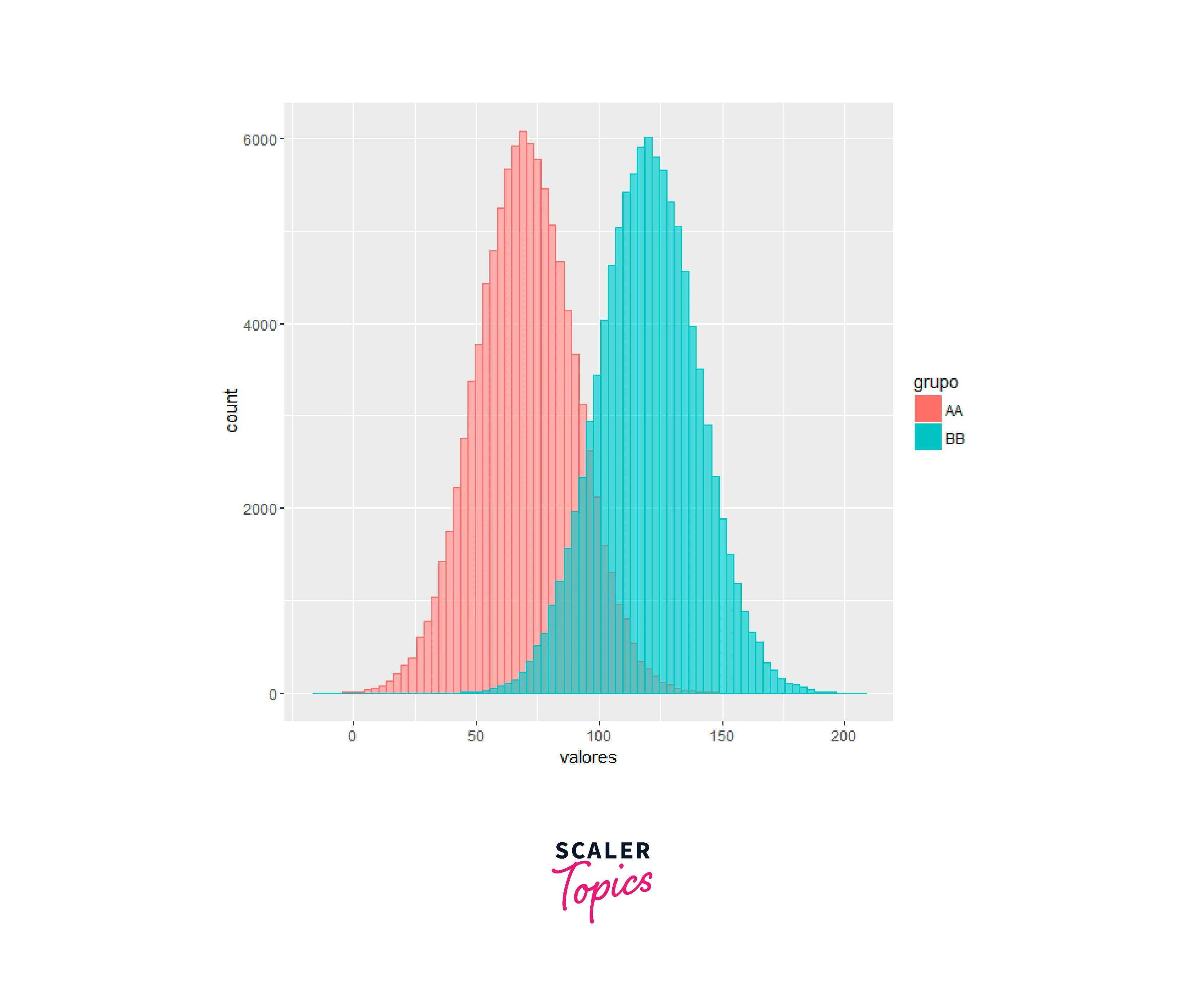
You can further enhance your visualization by using faceting to create separate plots for different groups within your data. This can be particularly useful when comparing distributions between groups.
In this example, the facet_wrap() function creates separate panels for different groups, allowing you to easily compare the distribution of value for each group.
By combining histogram and density plots, you can effectively visualize both the frequency distribution and the underlying smooth density estimation of your data. This approach provides a comprehensive understanding of your data's distribution characteristics and helps you make more informed data-driven decisions.
Customized Density Plots in R
Density plots are effective visualizations for understanding the distribution of continuous data. With the ggplot2 library in R, you can create customized density plots that highlight specific aspects of your data distribution. In this guide, we'll explore various customization options to create informative and visually appealing density plots.
- Step 1: Load the Necessary Libraries
Before you start, make sure you have the ggplot2 library installed. If not, you can install it using:Then, load the library:
library(ggplot2) - Step 2: Prepare Your Data
For illustration purposes, let's assume you have a dataset named data with a continuous variable named value. Replace this with your actual data and variable. - Step 3: Create a Basic Density Plot
Start by creating a basic density plot using the geom_density() function: - Step 4: Customization Options
Now, let's explore various customization options to enhance your density plot:- Change Line and Fill Colors:
You can use the scale_color_manual() and scale_fill_manual() functions to change line and fill colors, respectively. For example:
- Adjust Line Type and Size:
You can modify line type and size using the linetype and size aesthetics:
- Change Line and Fill Colors:
By exploring these customization options, you can create density plots that effectively communicate your data's distribution characteristics and emphasize specific features. Experiment with different combinations to create visualizations that suit your analysis goals and presentation preferences.
Interactive Bandwidth Choice
Interactive bandwidth choice transforms density plot visualization in R by allowing users to dynamically manipulate the smoothing bandwidth parameter. This pivotal control governs the plot's data smoothing degree, profoundly influencing its visual representation and information portrayal. Employing tools such as Shiny, users can seamlessly explore a spectrum of bandwidth values, aligning the visualization with their specific analytical requirements. This interactive functionality fosters a profound comprehension of data distribution traits, enabling users to instantaneously witness the diverse effects of different bandwidths on plot granularity and pattern discernment. By affording real-time bandwidth control, this method empowers users to unearth concealed insights, rendering density plots more insightful, interactive, and amenable to efficient data exploration and effective communication.
In this example, we're using the "mpg" dataset from the "ggplot2" package to create an interactive density plot of city miles per gallon (cty) values. Users can adjust the bandwidth parameter using a slider input, which dynamically updates the density plot.
Faceting and Grouping in Density Plots
Faceting and grouping are powerful techniques in density plot visualization that enable the exploration and comparison of data distributions across multiple dimensions. Faceting involves creating a grid of smaller plots, each depicting a subset of the data, based on categorical variables. This approach allows us to examine how the distribution of a continuous variable varies across different groups or levels within the categorical variable, providing insights into potential patterns or disparities.
Grouping, on the other hand, involves overlaying multiple density plots within a single plot, each representing a distinct group or category. By utilizing different line colors or fill patterns, grouping effectively juxtaposes multiple distributions, allowing for direct visual comparison. This is particularly valuable when analyzing how the density of a continuous variable differs among various groups, aiding in the identification of similarities, differences, and outliers.
In this example, the facet_wrap() function is used to create individual density plots for each species of iris flowers. The fill aesthetic assigns different colors to the species in the plot.
Combining faceting and grouping in density plots provides an enhanced ability to dissect complex data relationships. This approach can unravel hidden trends and patterns that may not be immediately apparent when examining a single plot. It allows for a deeper understanding of the distributional characteristics of data subsets, facilitating data-driven decision-making and hypothesis generation. Whether investigating multivariate data or exploring the impact of different factors on a variable's distribution, the synergy of faceting and grouping empowers analysts to extract richer insights and communicate findings more effectively through density plots.
Fill Area Under Density Curves
Density plots are effective tools for visualizing the distribution of continuous data. By filling the area under the density curve, you can enhance the clarity and emphasis of the distribution while also adding a visually appealing element to your plot. In this guide, we'll explore how to fill the area under density curves in R using the ggplot2 library.
- Step 1: Prepare Your Data
For illustrative purposes, let's assume you have a dataset named data with a continuous variable named value. Replace this with your actual data and variable. - Step 2: Create a Filled Density Plot
To fill the area under the density curve in a density plot, you can use the geom_density() function and specify the fill aesthetic. Here's how you can do it:In this example, the fill aesthetic is set to a constant value ("Density"), and the alpha parameter controls the transparency of the filled area. Adjusting the alpha value allows you to control the intensity of the fill color.
- Step 3: Combining Fill with Grouping
You can further enhance your plot by combining fill with grouping. For instance, if you have a categorical variable named group and you want to fill the density area for each group separately, you can do the following:
In this case, the fill aesthetic is set to the categorical variable group, allowing each group's density curve to be filled with a distinct color.
Filling the area under density curves adds visual emphasis to the distribution while aiding in the comparison of different groups. It enhances the readability of your plots and helps highlight the overall shape and characteristics of the data distribution. By experimenting with different fill colors, transparencies, and grouping options, you can create density plots that effectively communicate the underlying data patterns and insights.
Conclusion
- Density plots are powerful tools in R for visualizing the distribution of continuous data. They offer a smooth representation of data density, revealing underlying patterns and characteristics that may not be immediately apparent in other types of plots.
- Density plots in R, particularly when used with the ggplot2 library, provide extensive customization options. Users can adjust colours, line types, fill patterns, and more to tailor the plot's appearance to their specific needs and preferences.
- Density plots help in understanding the shape, central tendency, and spread of data distributions. By overlaying multiple density plots or using faceting and grouping, analysts can compare distributions across different categories, enabling deeper insights and data-driven decision-making.
- Integrating interactivity through tools like Shiny allows users to dynamically manipulate parameters such as bandwidth, enhancing the plot's adaptability and enabling real-time exploration of data smoothing effects.