Descriptive Statistics in Excel

Introduction to Descriptive Statistics in Excel

Your dataset is summarized using descriptive statistics in excel, which depicts the dataset's characteristics. These characteristics include different measurements of central tendency and variability, distributional characteristics, outlier detection, and other details. Descriptive statistics don't try to apply from a sample to a population like inferential statistics do; they describe the characteristics of your dataset.

Excel can generate descriptive statistics in excel for your dataset using just one function. Even if Excel isn't your main statistical software program, this piece is a great introduction to understanding descriptive statistics.

If the data analysis option is not visible on the data tab, follow the instructions in the following section to make it visible.

• Use graphs and descriptive statistics in excel together.
• The statistical output includes numerical representations of the characteristics of your data.
• Charts are frequently easier to understand while still providing useful information.
• The ideal method for maximizing understanding is to combine graphs with statistics results.
• We have shown the histograms for the variables in this dataset at the end of this article.

We'll evaluate two factors in this example, teenage girls' height and weight. These data were gathered during an actual experiment. Your data should be organized in columns or rows in Excel to use this feature. My data is organized into columns, as seen in the sample below.

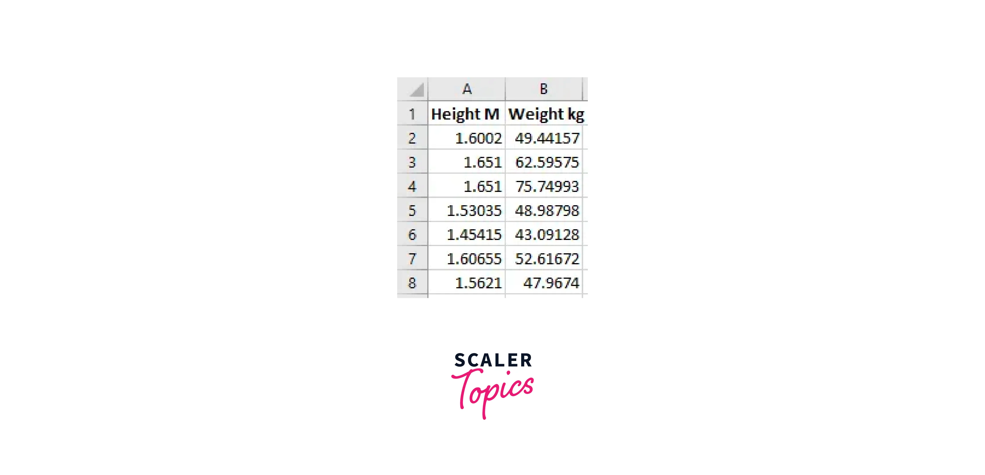
Download the HeightWeight Excel file to see the data for this example.

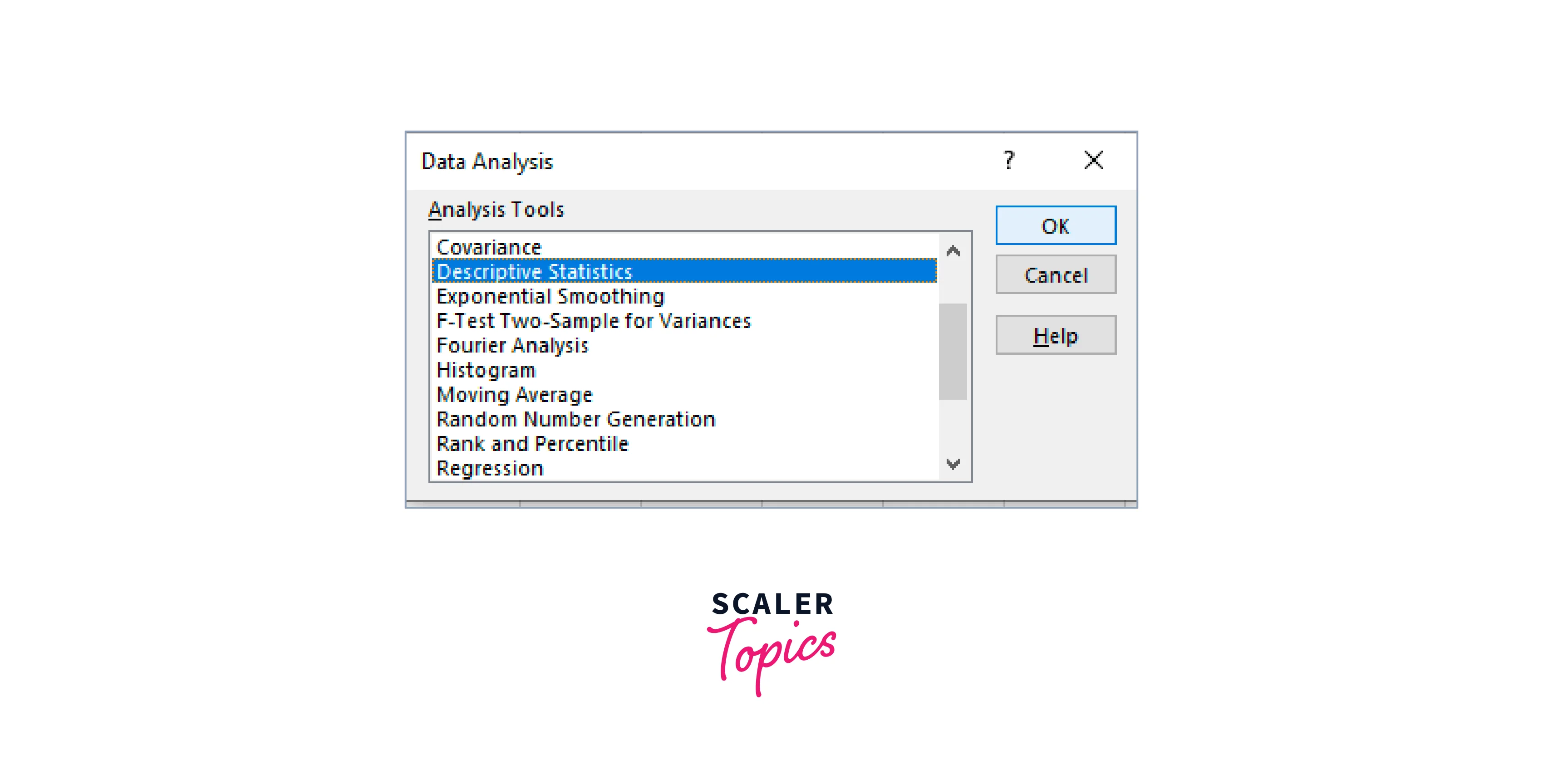
Click Data Analysis in Excel's Data tab, as indicated above. Select Descriptive Statistics in the Data Analysis box, then proceed as directed.

Instructions for Filling in Excel’s Descriptive Statistics Box

• Choose the range for the variables you want to analyze under Input Range.
• If they all fit into one block, you can use multiple variables.
• Although you can look at many variables, the analysis evaluates each one univariately (i.e., there is no association).
• Select the grouping of your variables in Grouped By. I always use the software-standard format of one variable per column.
• A different option is to use one variable per row.
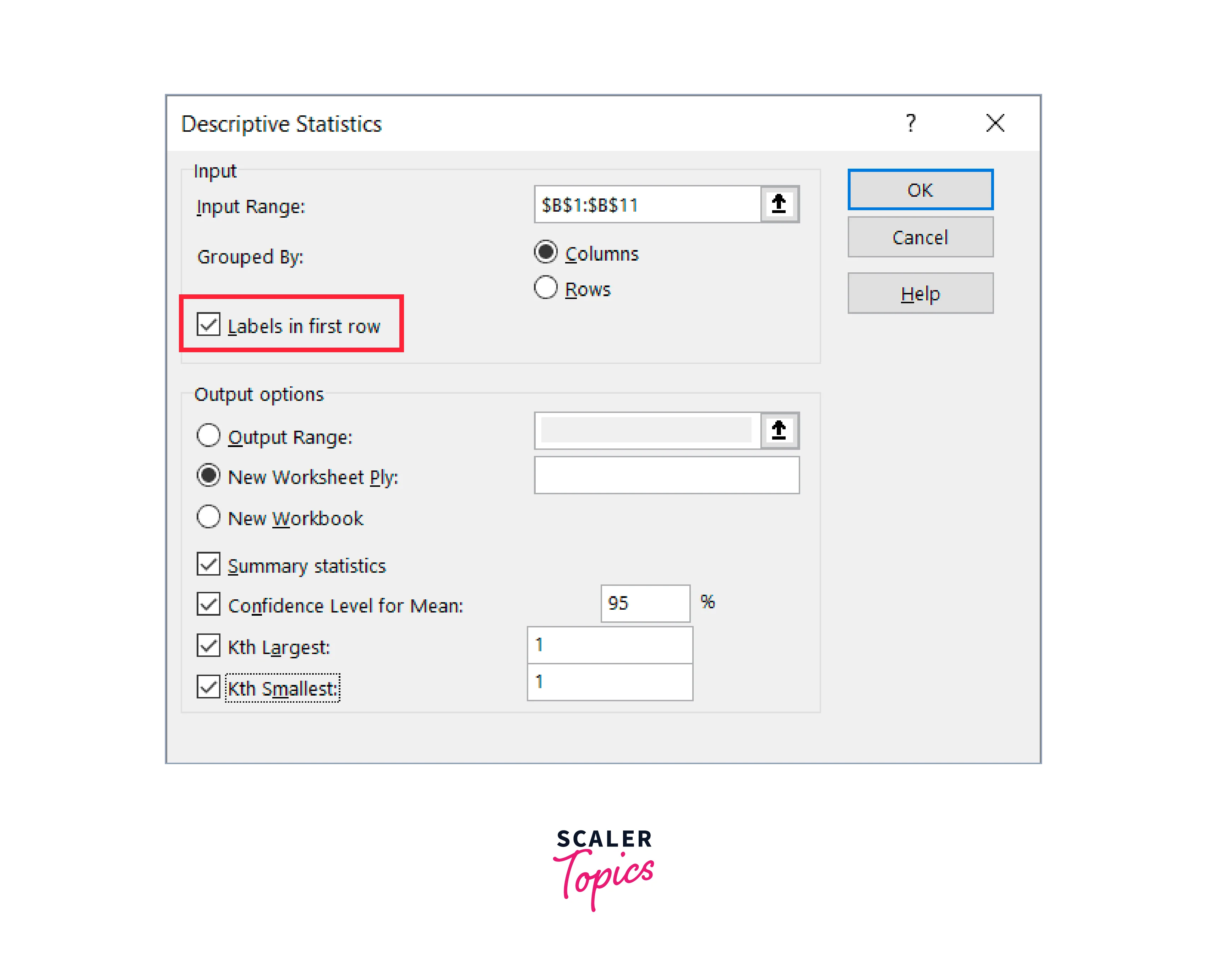
• If row 1's variable names are meaningful, check the Labels in the first-row box. With this selection, the output is simpler to understand.
• Choose where you want Excel to display the results in Output choices.
• To view most descriptive statistics (including central tendency, dispersion, distribution characteristics, total, and count), check the Summary statistics box.
• To get a confidence interval for the mean, check the Confidence Level for the Mean box. Enter your degree of confidence. Usually, a good value is 95%. Read my post on confidence intervals for additional details regarding confidence levels.
• To show a high and low value, check Kth Largest and Kth Smallest. Excel shows the maximum and lowest values.
• Select OK.
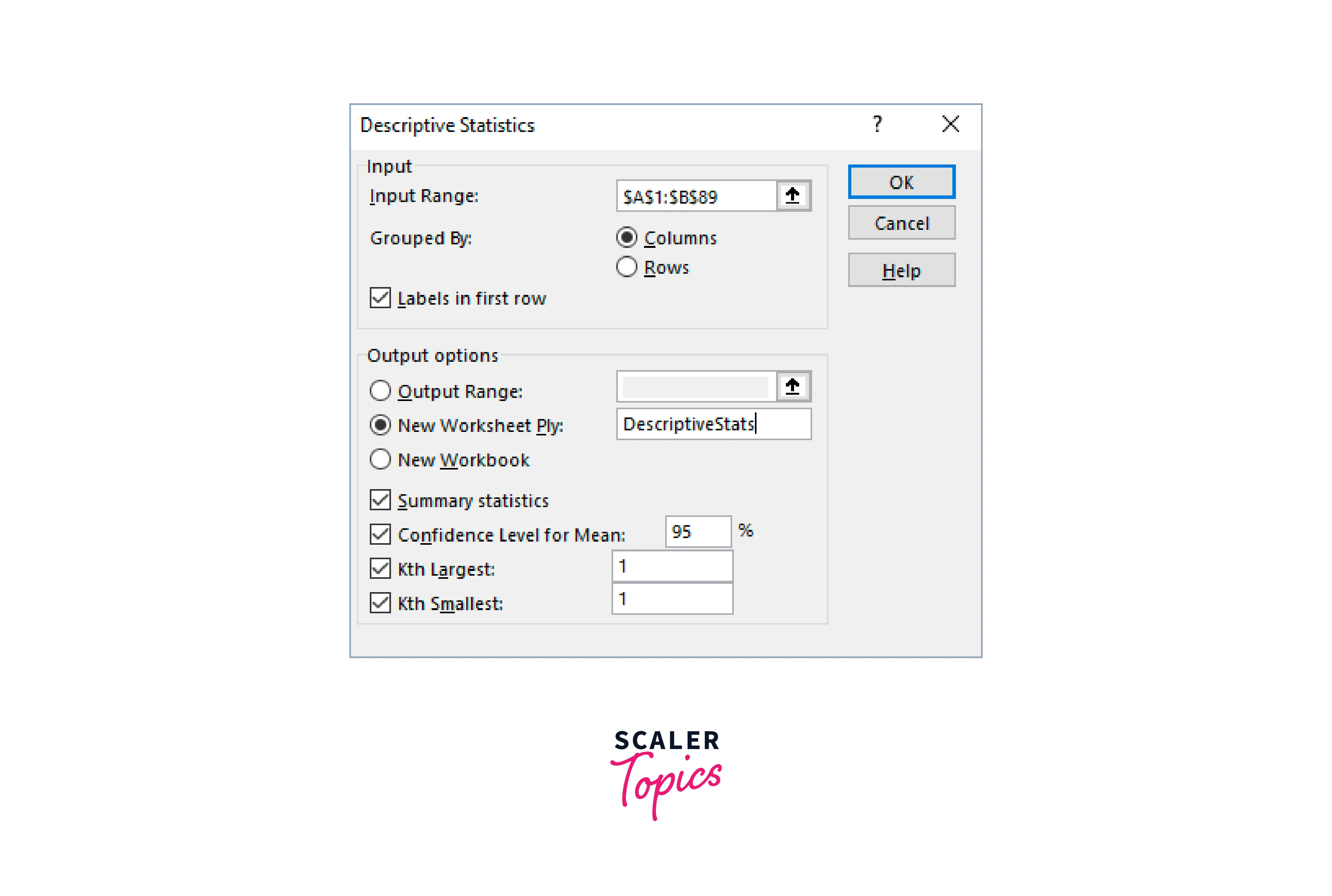
• Fill out the dialogue box as indicated below for our example dataset.

How to Get Descriptive Statistics in Excel?

To extract descriptive statistics in excel we would first need enable the Data Analysis Toolpak in Excel.

The various steps to enable the Data Analysis Toolpak in Excel are as follows:

Step 1: Launch any Excel file. Go to the File tab.

Step 2: Select Options. The Excel Options dialogue box will appear as a result.

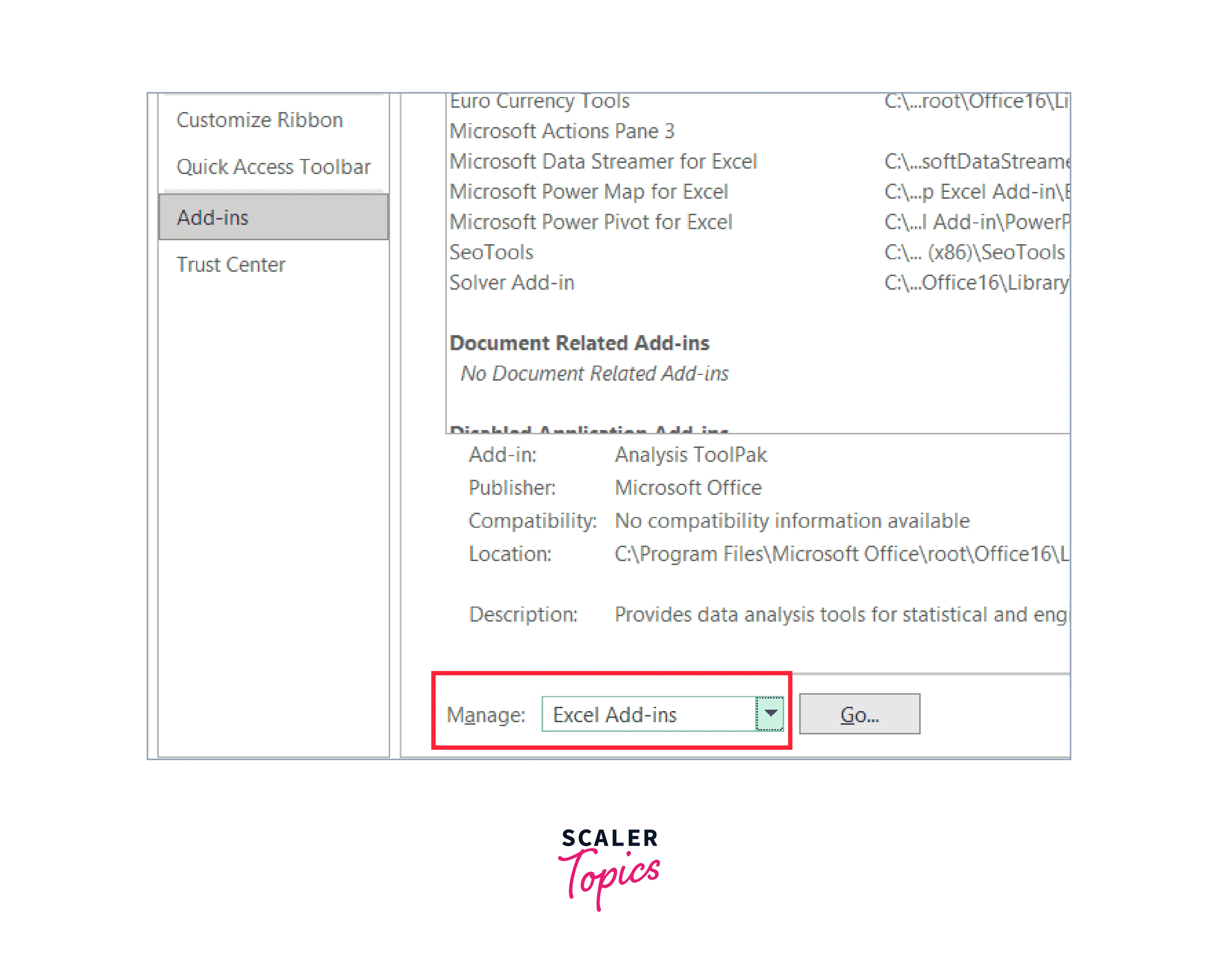
Step 3: In the left pane of the Excel Options dialogue box, select Add-ins.

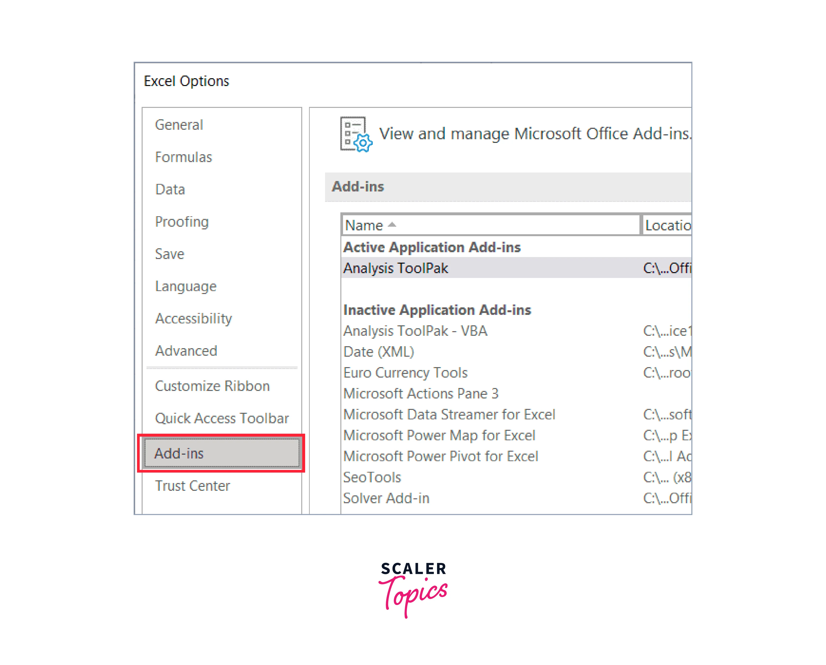
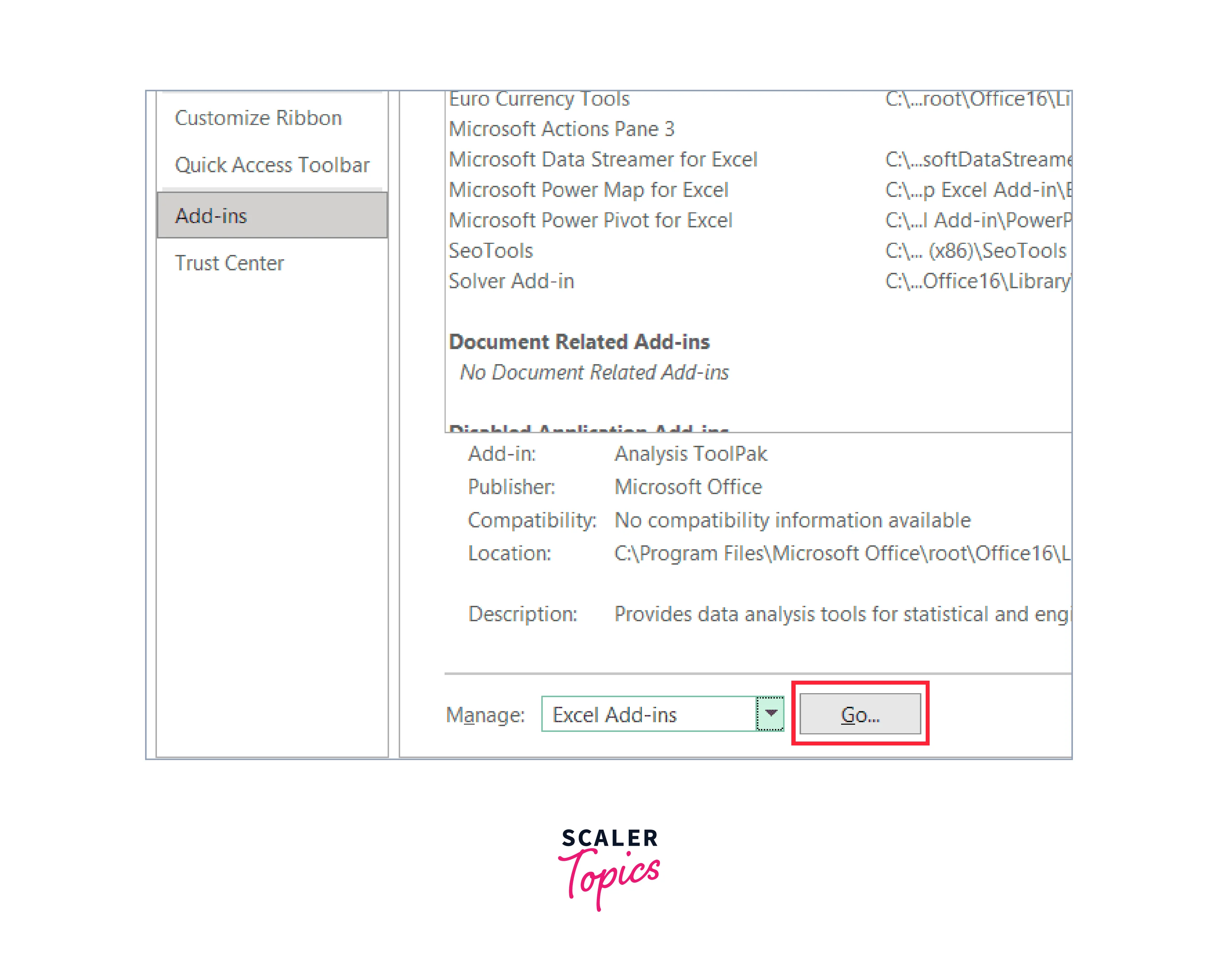
Step 4: Select 'Excel Add-ins' from the Manage drop-down menu that is located at the bottom of the dialogue box.

Step 5: Press the "Go" button.

Step 6: Check the Analysis Toolpak box when the Add-ins dialogue box appears.

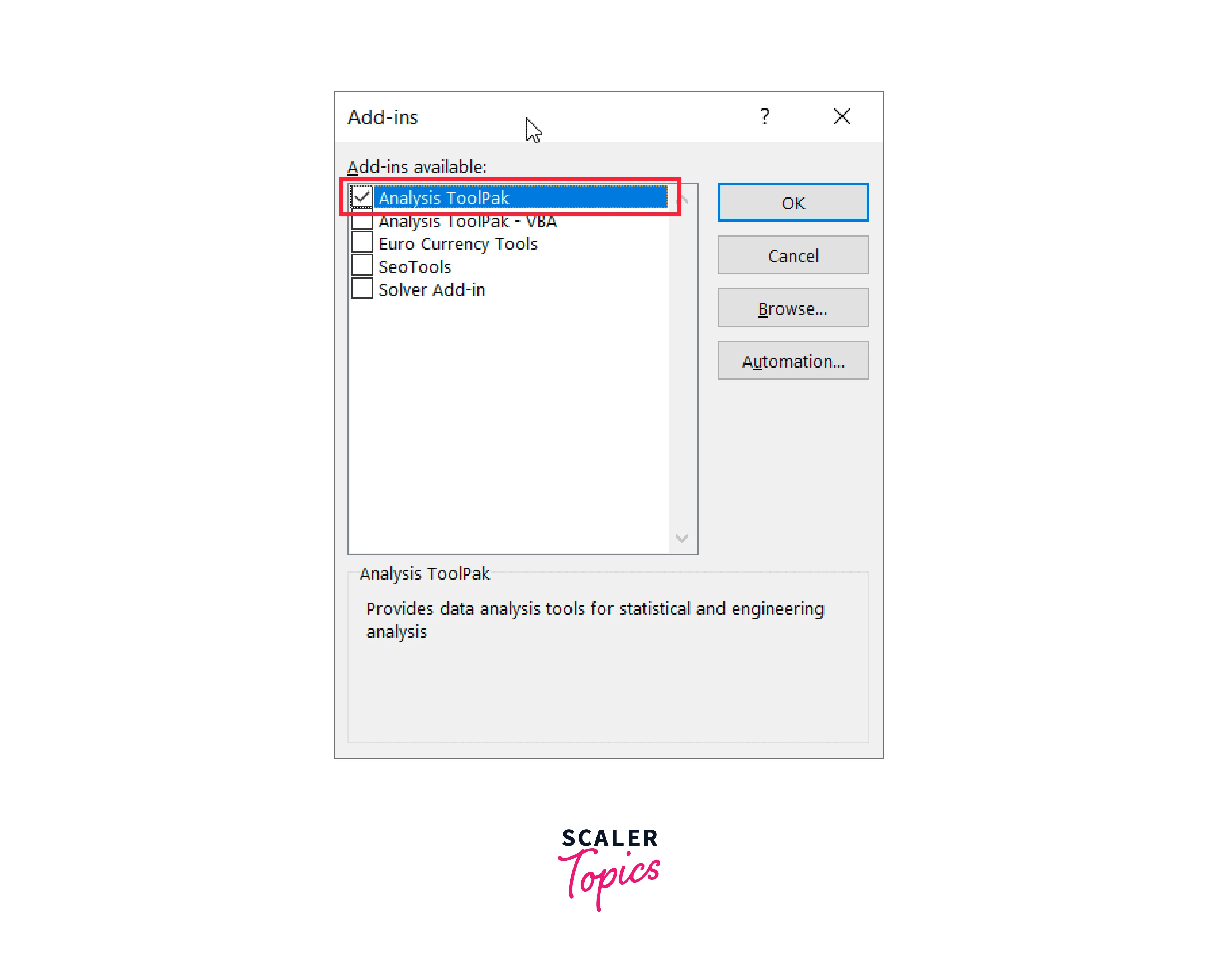
Step 7:

• Click OK.
• All your Excel workbooks can use the Data Analysis toolpak once the remaining steps have been completed.
• Now that it has been activated let's look at how to obtain descriptive statistics using the Data Analysis Toolpak.
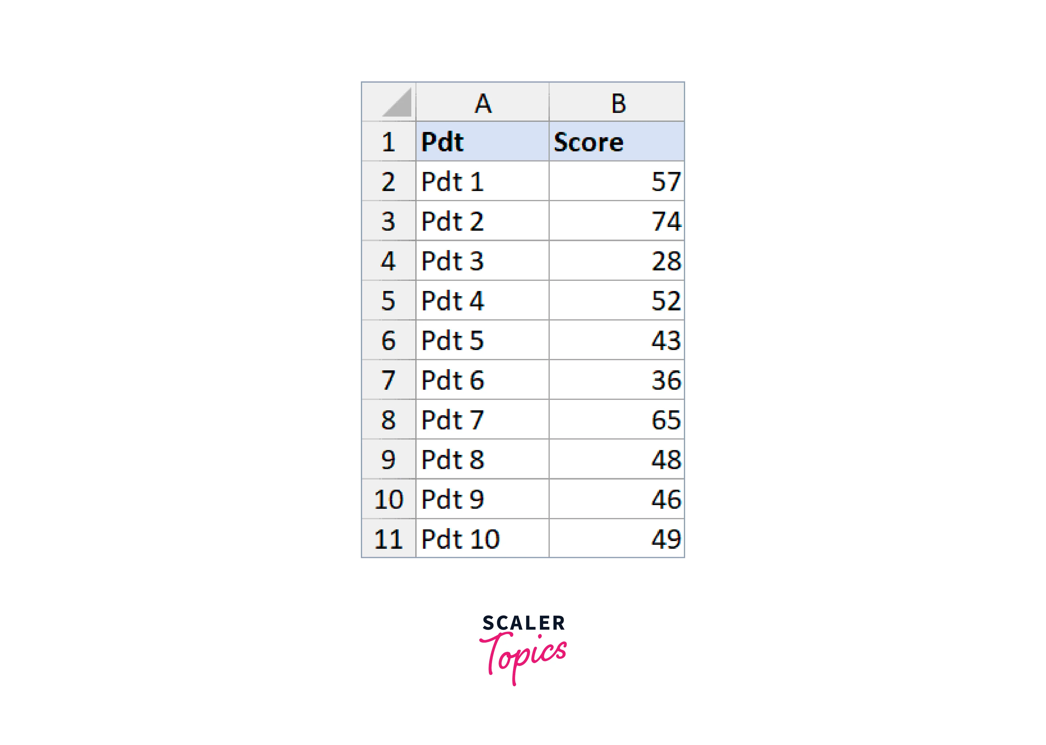
• Assume you have the data set below, which contains sales information for several products a corporation sells. For this data, I want to get descriptive statistics.

The procedures are as follows:

• Go to the Data tab.
• Click Data Analysis under the Analysis category.
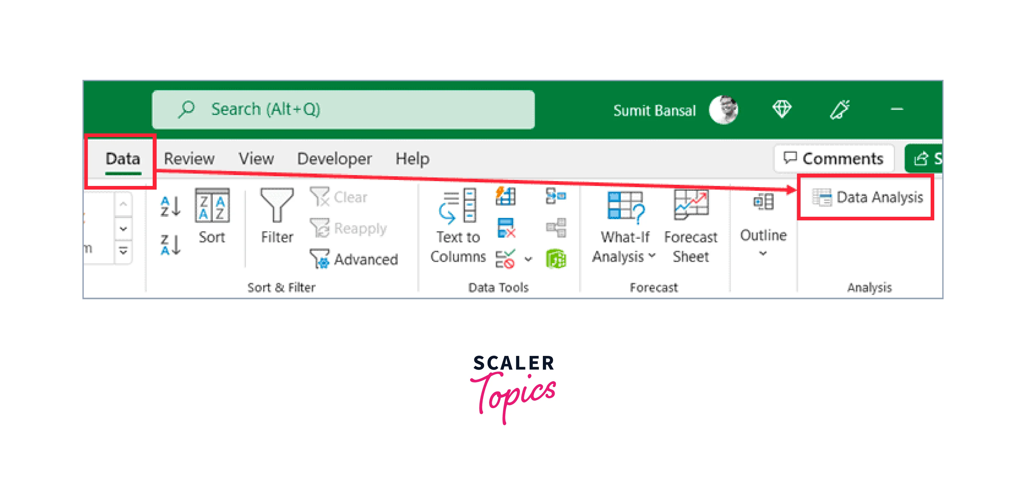
• Select Descriptive Statistics from the Data Analysis dialogue box that appears.
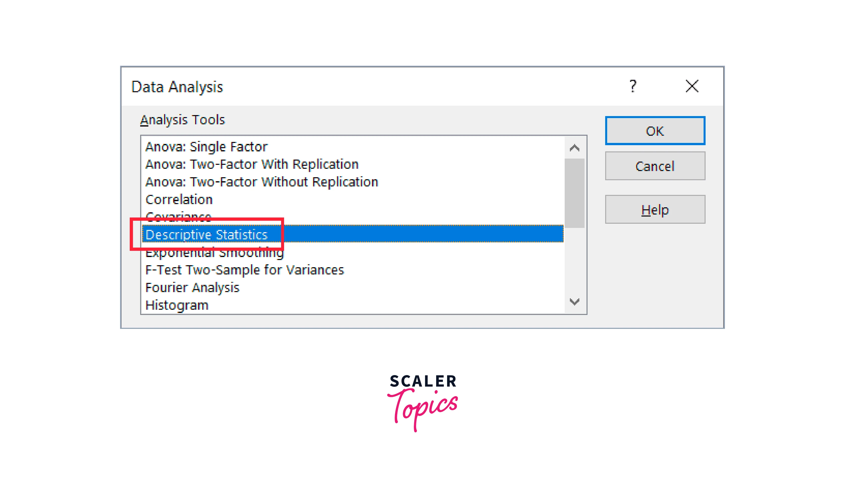
• Click OK
• Enter the data's input range in the Descriptive Statistics dialogue box. Because this input only accepts numeric data, please note that I have only used Column B as the data source.
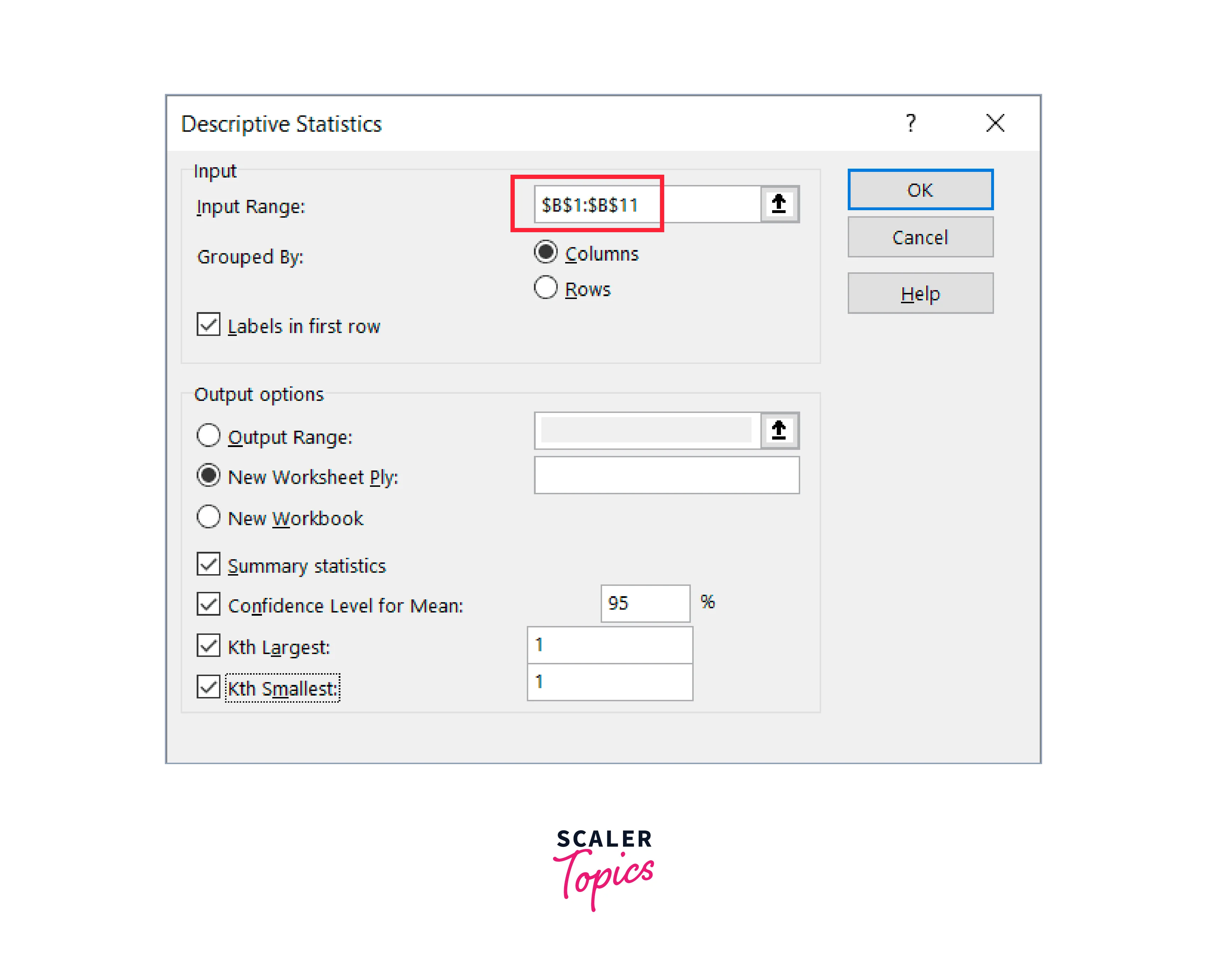
• If your data includes headers, select "Labels in first row."
• Choose the option for New Worksheet Ply to receive the result on a new sheet.
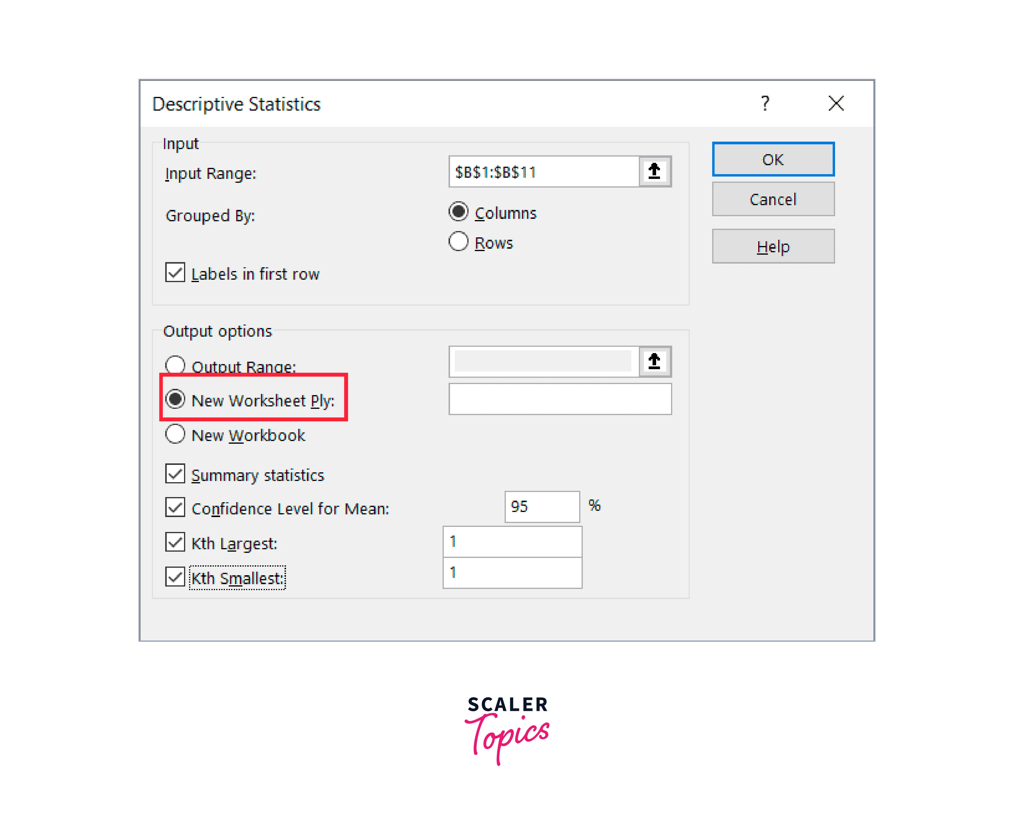
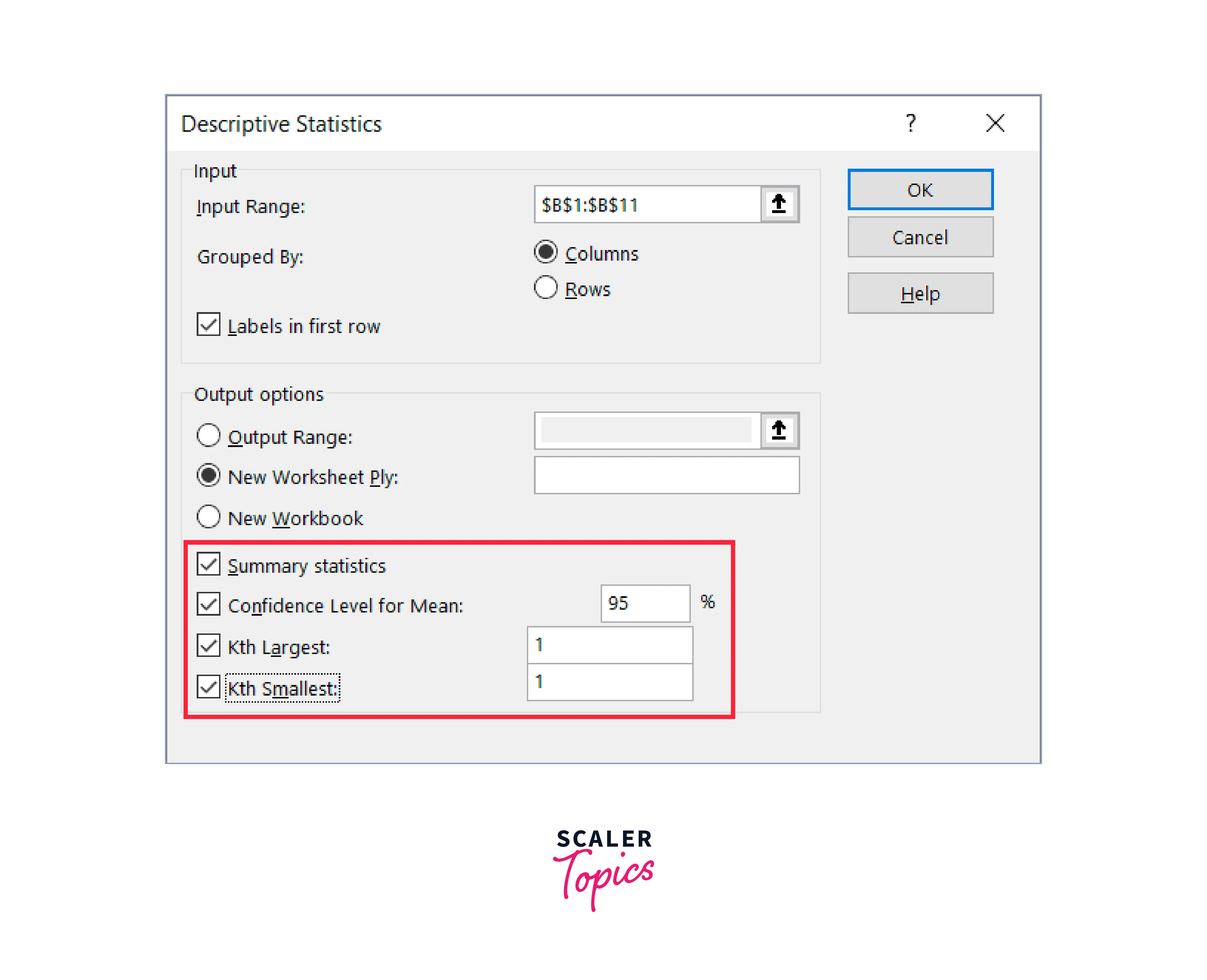
• Choose the statistics choices you'd want to use (you must choose at least one, but you may choose all four).
• Click OK
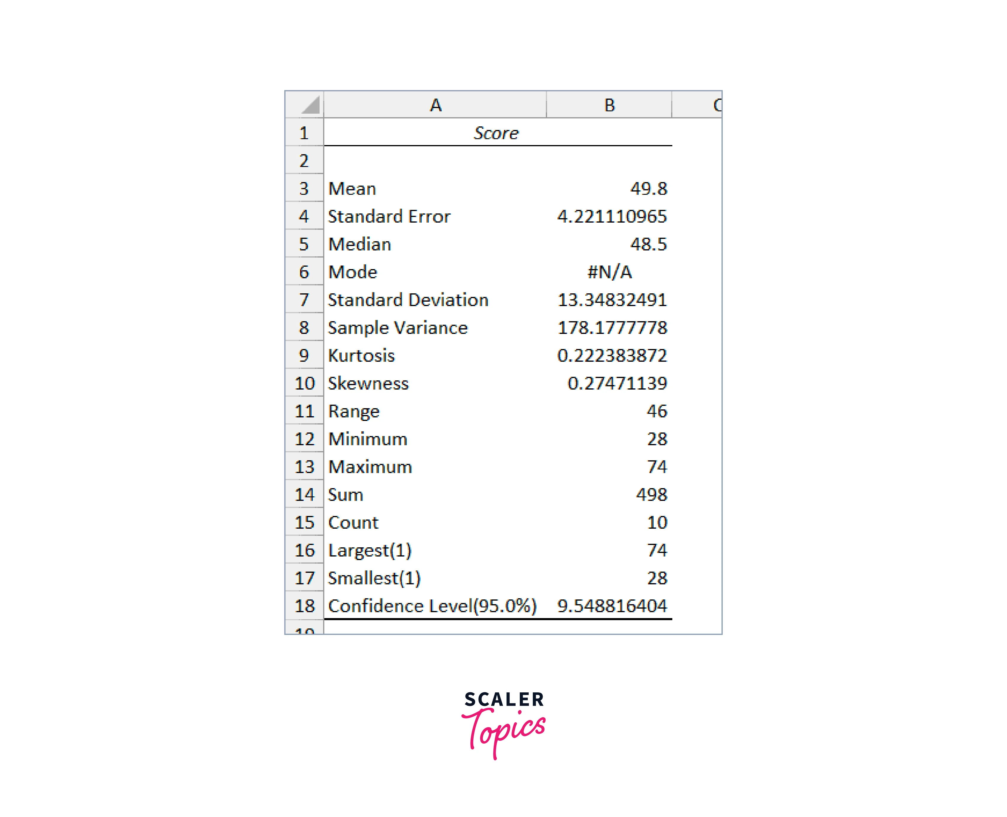
• By following the instructions above, a new sheet will be inserted, and you will receive the statistics displayed below:

Be aware that step 8 allows you to define the following:

• The default value for the confidence level for the mean is 95%, but you can vary it.
• The default value for Kth Largest is 1, but you can modify it. If you enter 3, you will receive the dataset's third-largest value.
• The default value for Kth Smallest is 1, but you can modify it. If you enter 3, you will receive the dataset's third-smallest value.

Keep in mind that the values you receive as a result are static.

You must repeat the preceding steps if your original data changes and you want more descriptive statistics.

Thus, this is a convenient way to import descriptive statistics in excel.

Interpreting Excel’s Descriptive Statistics Results

Excel generates the statistical results, and I autofit the columns to make them more readable.

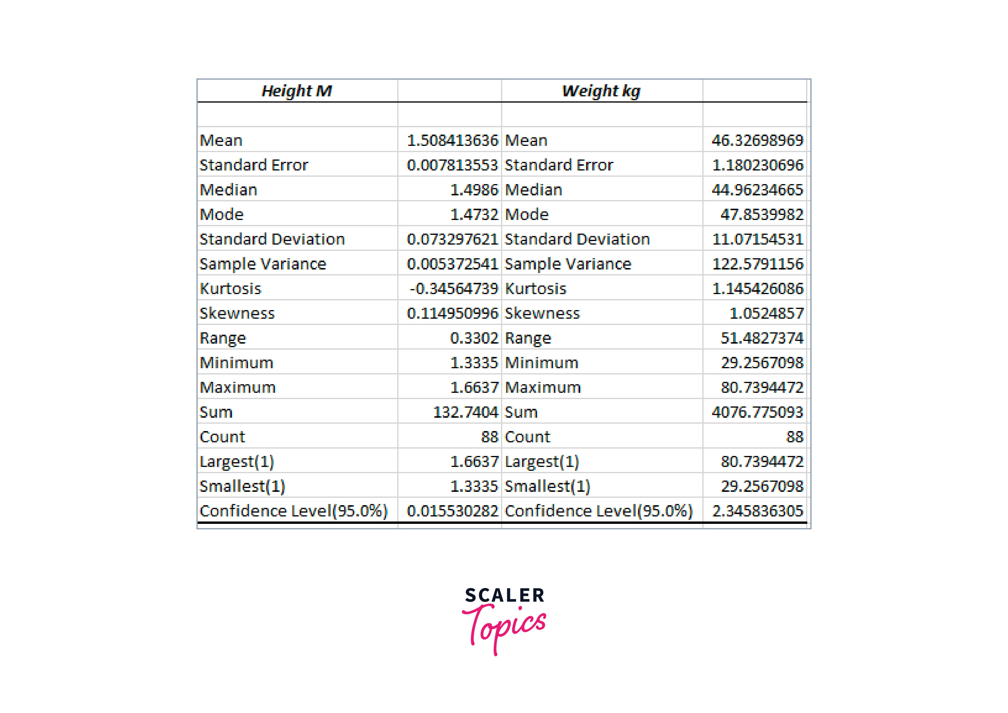
As you can see, we are evaluating two factors: kilogram weight and height in meters.

Typically, we'll start at the top of Excel's descriptive statistics output and work our way down. But I'll sort the outcomes into sensible categories. As a result, the order of the following conversation doesn't exactly match the output. Click the links for more in-depth information to learn more about the data.

Central Tendencies (Mean, Median, Mode)

Where the majority of the values in the dataset are found is indicated by a measure of central tendency. It sits in the middle of the range of values. Excel provides three central tendency measures. What is the best option for your data?

• Mean:
  It is mostly used for this measurement. It is calculated by dividing the total number of observations by their number. It works best with symmetrically distributed data.
• Median:
  The median divides your data in half. Half of the results are higher than the median, and the other half are lower. For skewed distributions, it works best.
• Mode:
  The value that appears most frequently in your data is represented by this measurement. For categorical and ordinal data, it works best.

The example data are continuous variables. Excel typically displays "N/A" for the mode when you have continuous data. This occurs since continuous data are unlikely to include values that perfectly replicate each other, which is necessary for the mode.

What can we infer from comparing the two variables' median and mean? They are nearly equal in height, measuring 1.51 and 1.50 meters, respectively. The mean and median will be quite near in symmetric distributions. That suggests that the heights have a symmetric distribution, which favors the mean. The height dispersion is centered around 1.51 meters, according to the mean.

The weighted median (44.9kg) and mean (46.3kg) do not match. A right-skewed distribution is shown when the mean is higher than the median. For these data, the median should be used. The data points are split evenly between those above and below 44.9kg.

Measures of Dispersion (Standard Deviation, Variance, Range)

You have already seen how a measure of central tendency shows where most observations fall. Dispersion measurements show how tightly or loosely distributed the data points are around the center. Excel provides three dispersion measures. Data points often move farther from the center as their values rise (the distribution widens).

• The standard deviation is the normal or average difference between each data point and the mean. By using the data's original units, this metric makes interpretation simpler. As a result, this measure of variability is the one that analysts utilize the most. The variance's square root yields the standard deviation.
• Variance is the average square of the values' deviations from the mean. The variance is expressed in squared units rather than the original data units because the calculations use squared differences. Although larger variance numbers signify greater variability, there is no logical explanation for certain values.
• The range is the difference between a dataset's largest and smallest values. The range is simple to comprehend, but it is highly prone to outliers because it is based simply on the two most extreme values in the dataset. The amount of the dataset also impacts the range. The range tends to widen as the sample size rises. Therefore, only compare variability using the range when the sample sizes are comparable.

Use the standard deviation typically. Consider using the interquartile range (IQR), which Excel sadly lacks when your data is somewhat skewed.

Distribution Shape Properties: Kurtosis and Skewness

Two measurements that aid in understanding the fundamental characteristics of the distribution of your data are kurtosis and skewness. These metrics assess how closely your distribution resembles the normal and symmetric distribution.

If either kurtosis or skewness deviates from zero, this suggests that the distribution of your data is not normally distributed. To determine that, utilize a normality test or a normal distribution plot.

Histograms show the same information more understandably. Even though these statistics are fully objective, graph axes and bin sizes can be changed to emphasize or downplay certain traits.

Kurtosis shows how your distribution's peaks and tails compare to the normal distribution. Does the peak differ from the normal distribution in height or length? The tails are either thicker or narrower. The blue distributions in the table have 0 kurtosis values for comparison, but the red distributions contain positive and negative kurtosis values.

Kurtosis value	Description	Graph
Zero	Consistent with a normal distribution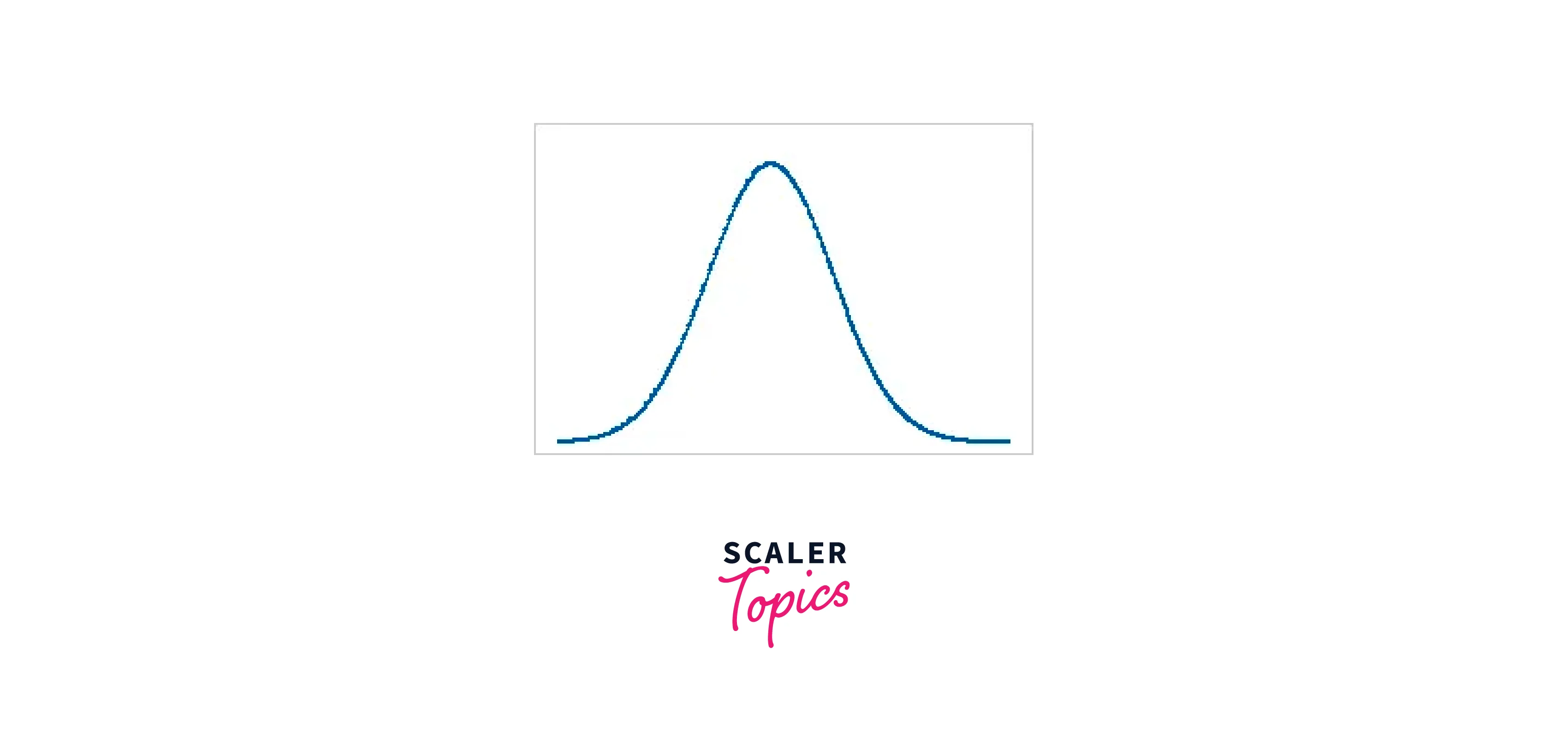
Positive	greater peak and narrower tails than the distribution's mean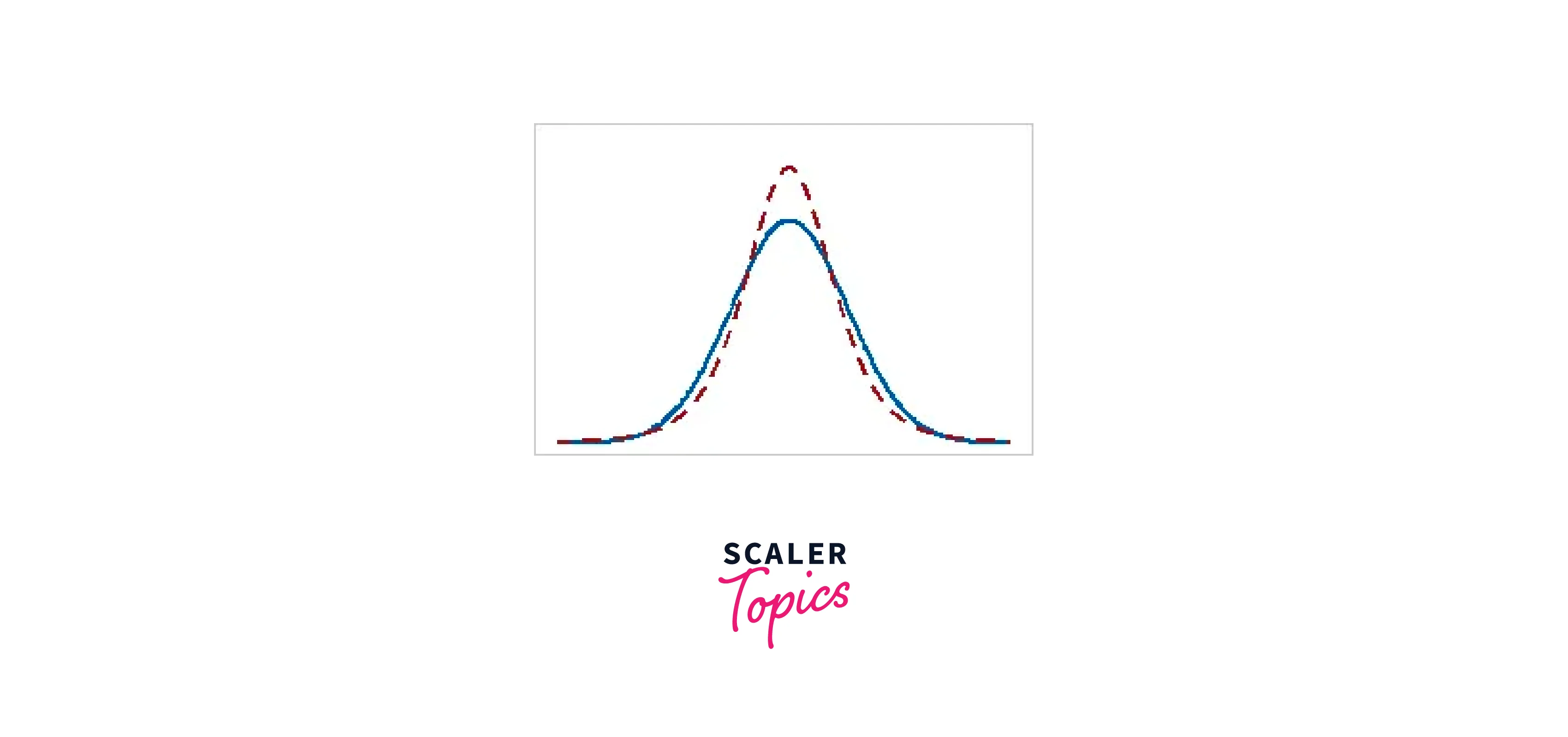
Negative	thinner tails and a shorter apex compared to the typical distribution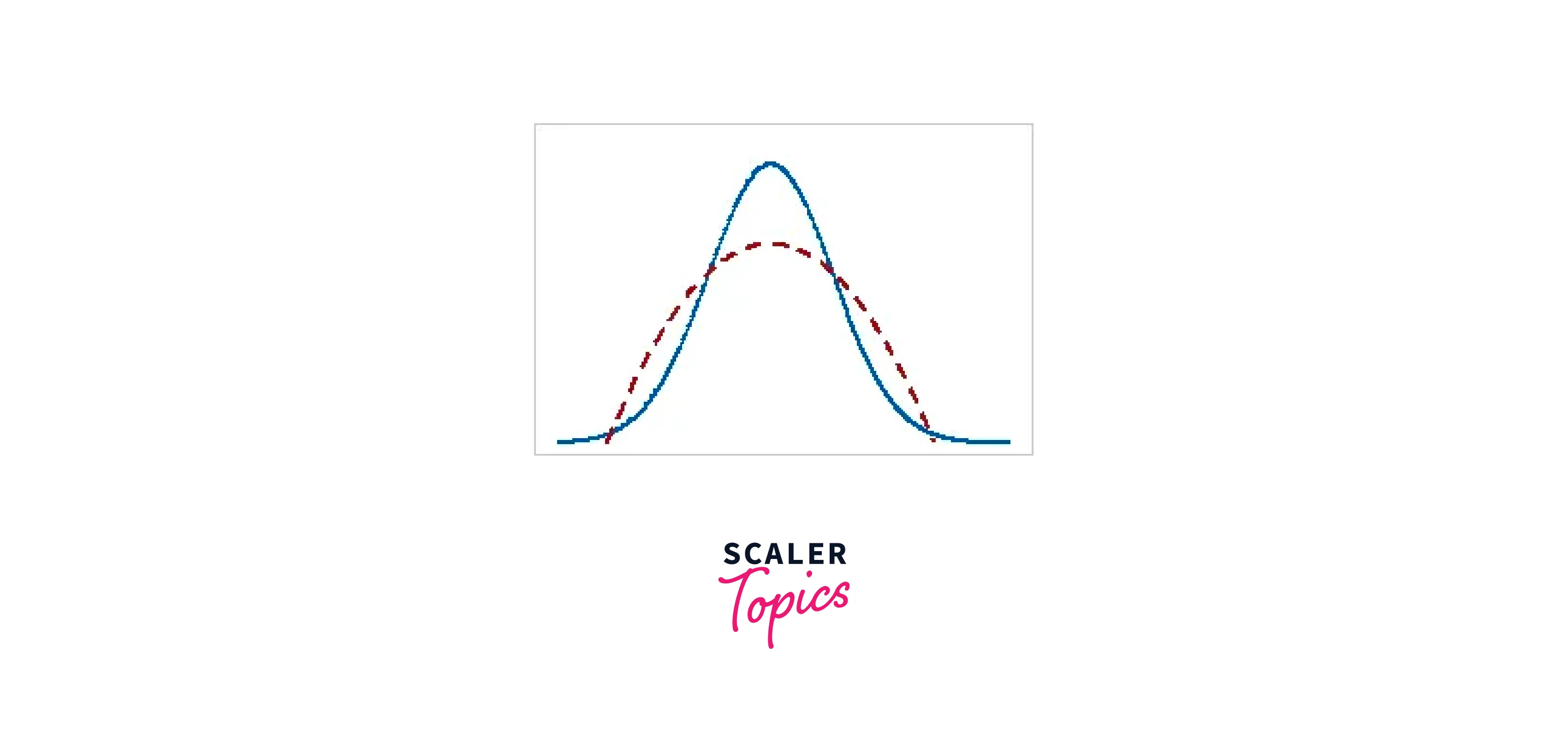

Height in our sample data has a kurtosis of -0.35. Indicating that the tails are consistent with the normal distribution, this number is very close to zero. Weight, on the other hand, has a kurtosis of 1.15, indicating that the tails are not as thick as they should be.

The skewness of your data reveals the symmetry of its distribution. Asymmetric data are skewed. On a distribution curve, the direction in which the long tail points are denoted by the words right-skewed and left-skewed.

Skewness value	Description	Graph
Zero	A perfectly symmetric distribution
Positive	Right-skewed data
Negative	Left-skewed data

A U-shaped distribution is inverted relative to the normal distribution but can still be symmetric.

The height variable in our example data has a skewness of 0.11. Since this number is nearly 0, the distribution of these data is symmetric. Weight, on the other hand, has a skewness of 1.05, indicating that it is right-skewed.

These distributional characteristics and the respective positions of the mean and median give a consistent picture of these two variables. Kurtosis and skewness are practically zero, while the mean and median for the height data are almost equal. All these measurements show that the heights exhibit a symmetric distribution compatible with the normal distribution.

In contrast, the weight data contain positive skew, positive kurtosis, and a mean higher than the median. These numbers imply that the weights deviate from the normal distribution by following an asymmetric, right-skewed distribution.

Minimum and Maximum

You may determine where your data fall by looking at your dataset's minimum and maximum values. For our example data, the weight ranges from 29.26 to 80.74 kg, and the height ranges from 1.33 to 1.66 M. These data can also be used to spot outliers. Data entry mistakes can result in values outside the acceptable range of information. See if the lowest and maximum figures make sense, given your data, by looking at them.

Sum and Count

The sum is the total of each variable's values. This has never been useful to me, but maybe it will be for you. The count represents how many observations there are for each variable. Check whether the sample size matches your expectations using this number. There are 88 observations for the weight and height variables combined.

Precision of the Mean: Standard Error and the Confidence Interval

The confidence interval and standard error measure how accurately your sample mean predicts the population means. Your sample estimate is most likely close to the actual population value if it is relatively accurate. On the other hand, a rough estimate is more likely to be off by a larger margin.

Since they use your sample data to infer the characteristics of a broader population, neither of the values technically belong in the output of the descriptive statistics (inferential statistics). Without taking the population into account, descriptive statistics just describe your data. I'll interpret them here because Excel includes them in the result.

Remember that inferential statistics constrain data collection techniques that descriptive statistics do not. For instance, these measurements are useless if you don't employ a representative sampling technique, like random sampling.

Histograms of our Descriptive Statistics Data

Check out the histograms for the data from our example. The descriptive statistics in Excel do not apply to these graphs. However, I advise you to graph your data before studying the numbers. The data used to generate the graphics below are described by the statistics on this page.

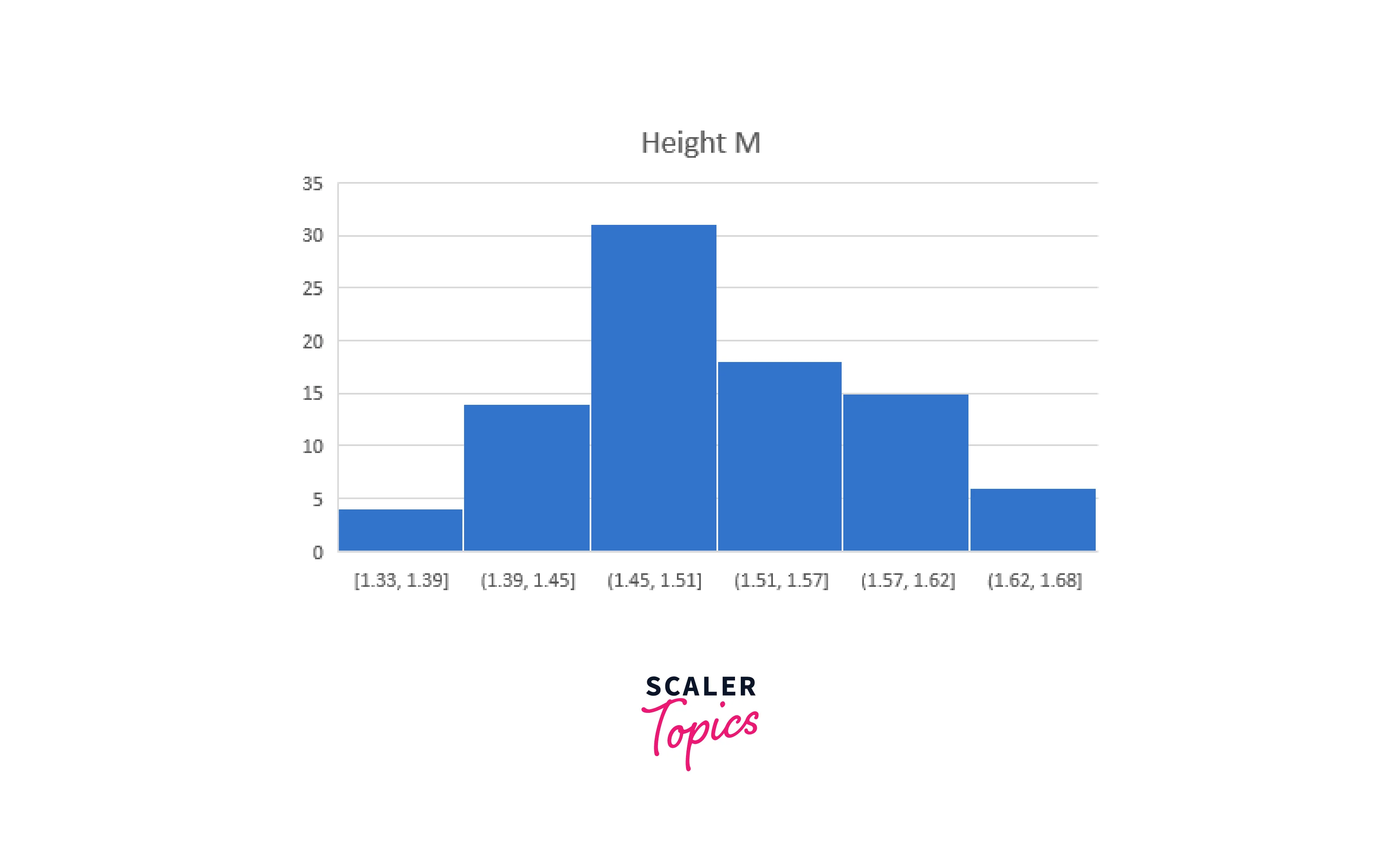
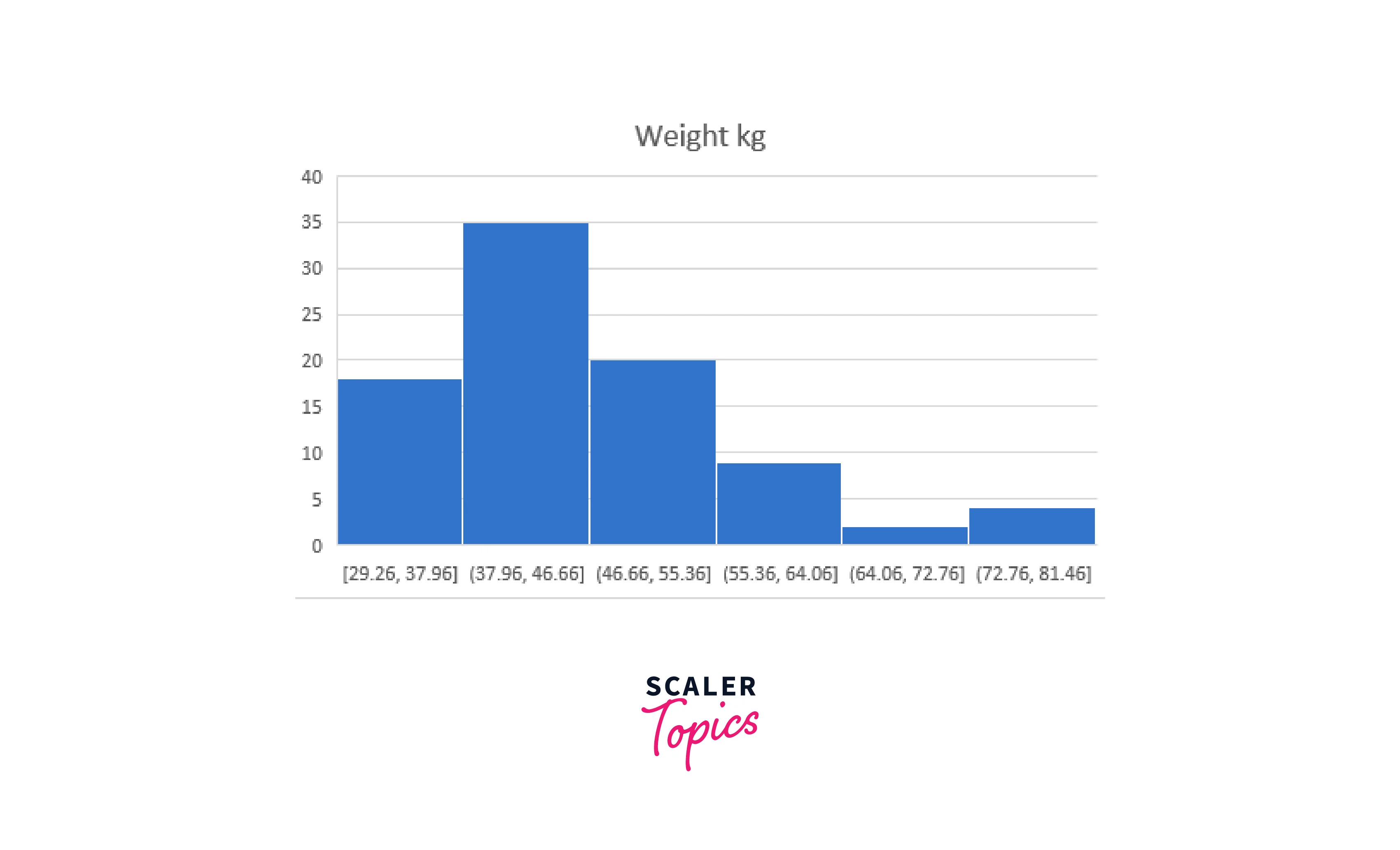
For my part, I expected the height information to be more symmetrical. However, they have a very slight rightward bias. The descriptive statistics are consistent with the weight data being more right-skewed.

Examples

We'll take a look at a few complex Excel Descriptive Statistics cases.

Example 1

Let's now examine some simple test data that comprises the results of 10 students. We need descriptive statistics to analyze the scores' data.

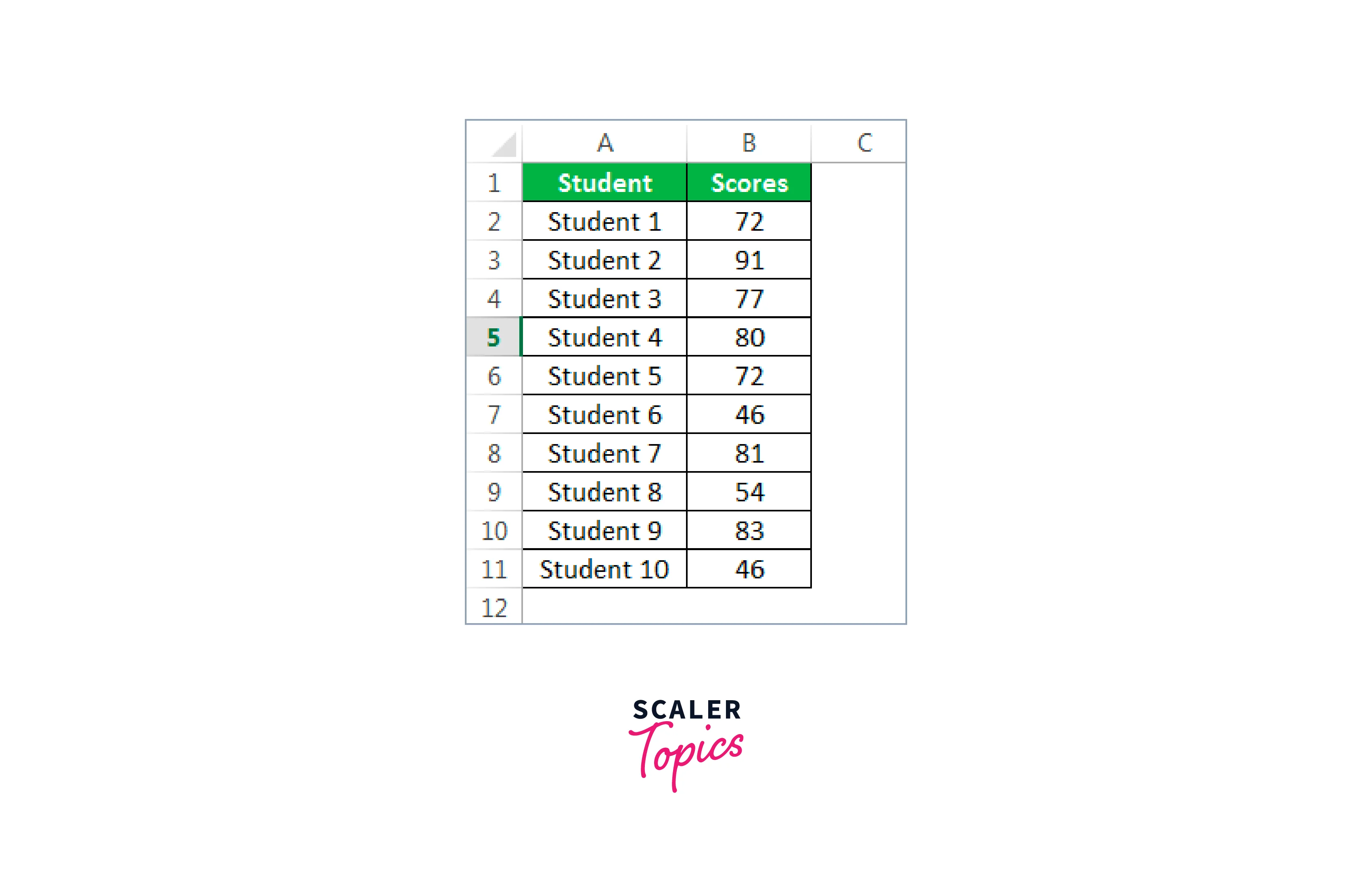
This information must first be copied to our Excel sheet.

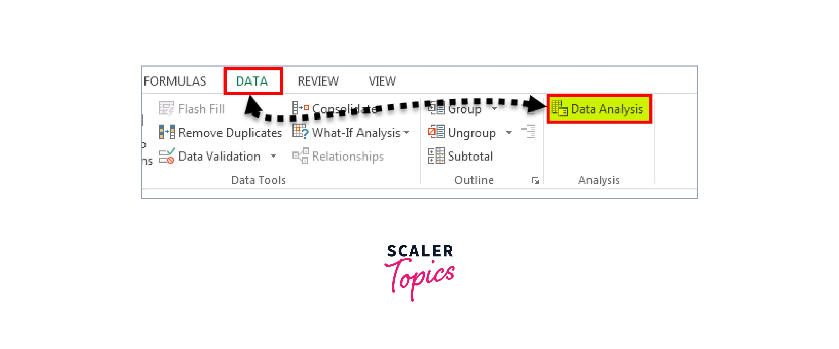
Step 1:
First, select Data, then Data Analysis.

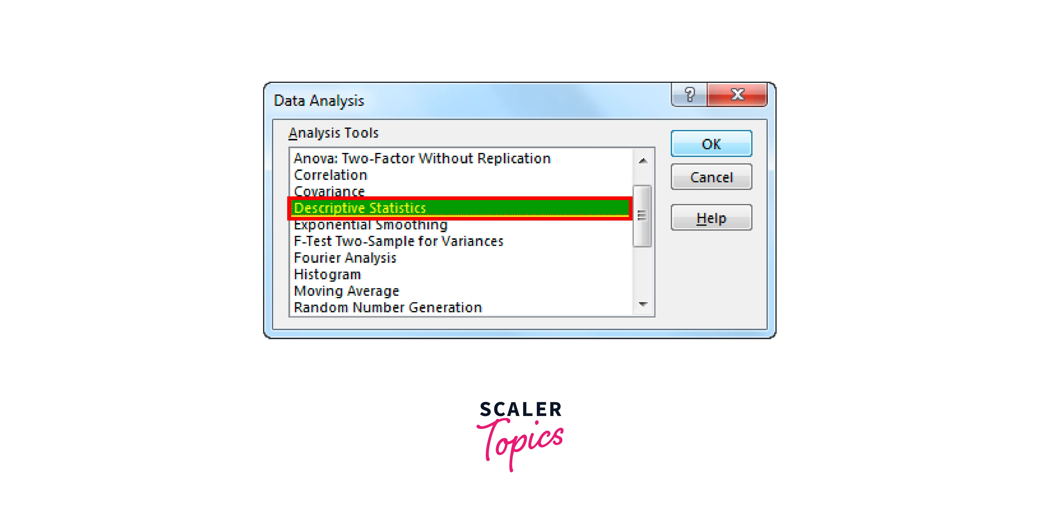
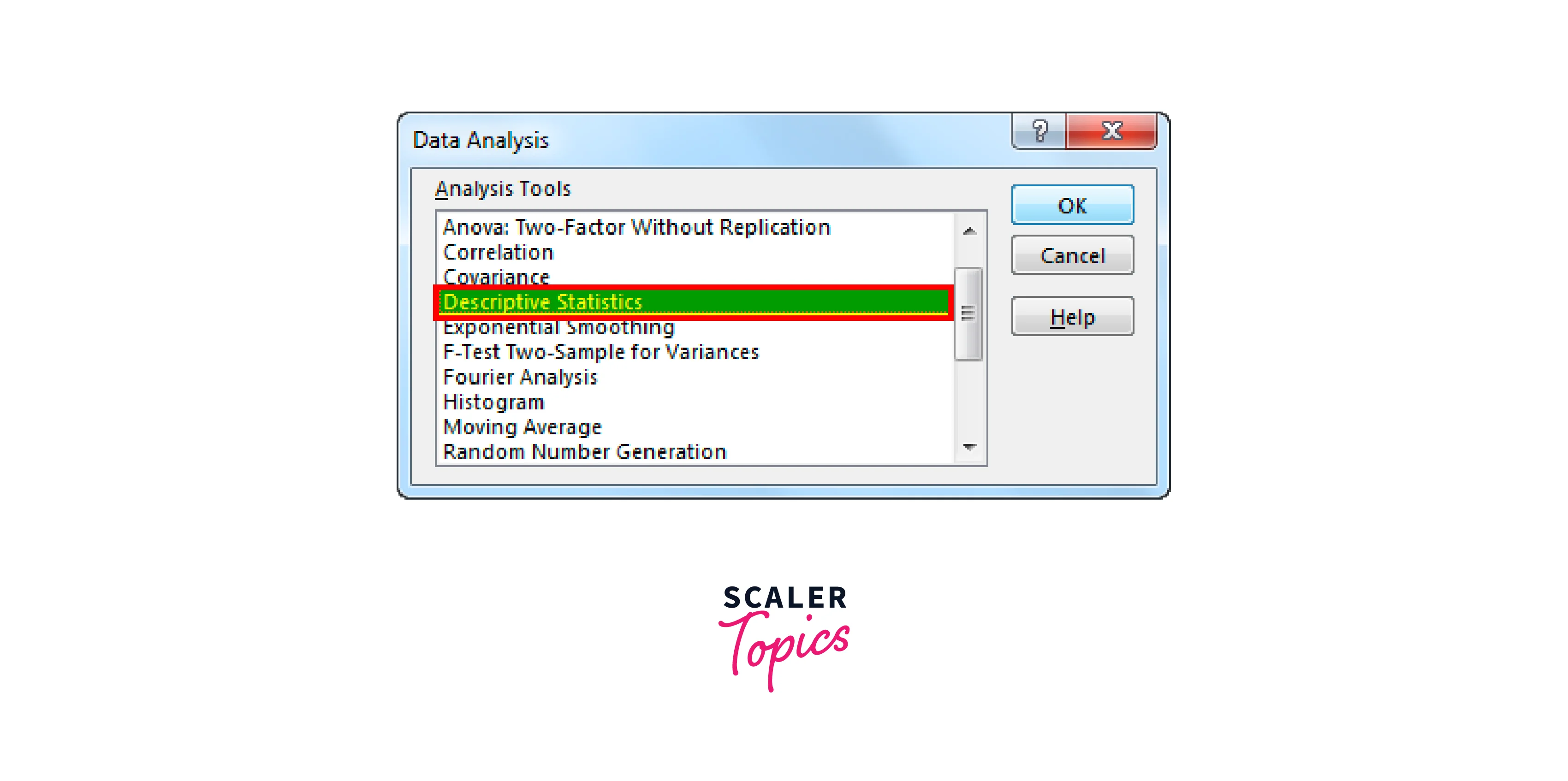
Step 2:
By selecting "Data Analysis," we are presented with a list of all the available analysis methods. After that, pick "Descriptive Statistics" by scrolling down.

Step 3:
Choose the "Scores range," including the header, under "Input Range." Next, select "Output Range," specify "Cell Reference" as "D1," check summary statistics, and ensure that "Labels in the first row" is selected.

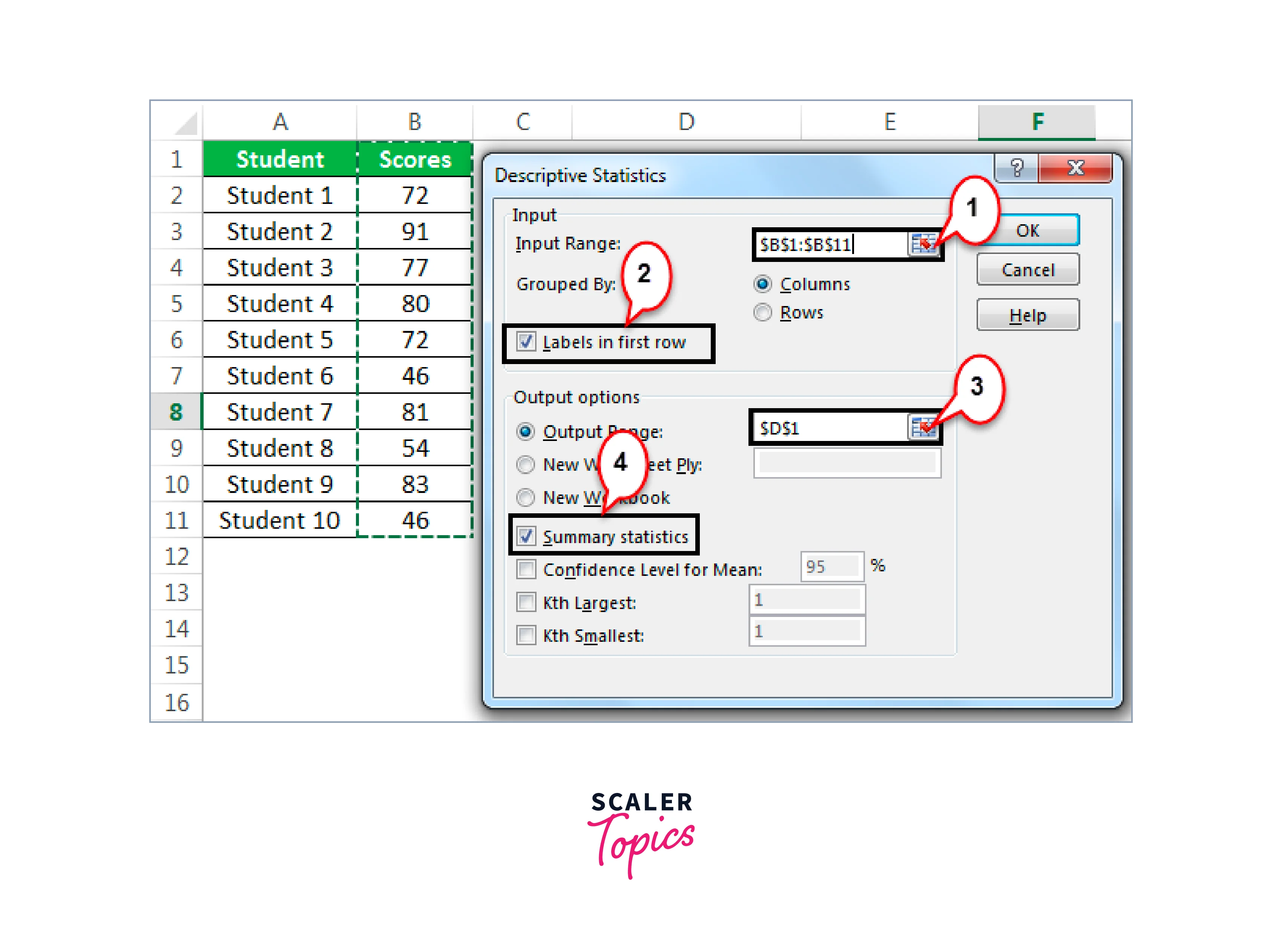
Step 4:
To finish the process, click "OK" at this point. We can see the executive summary of the descriptive statistics data analysis in the D1 cell.

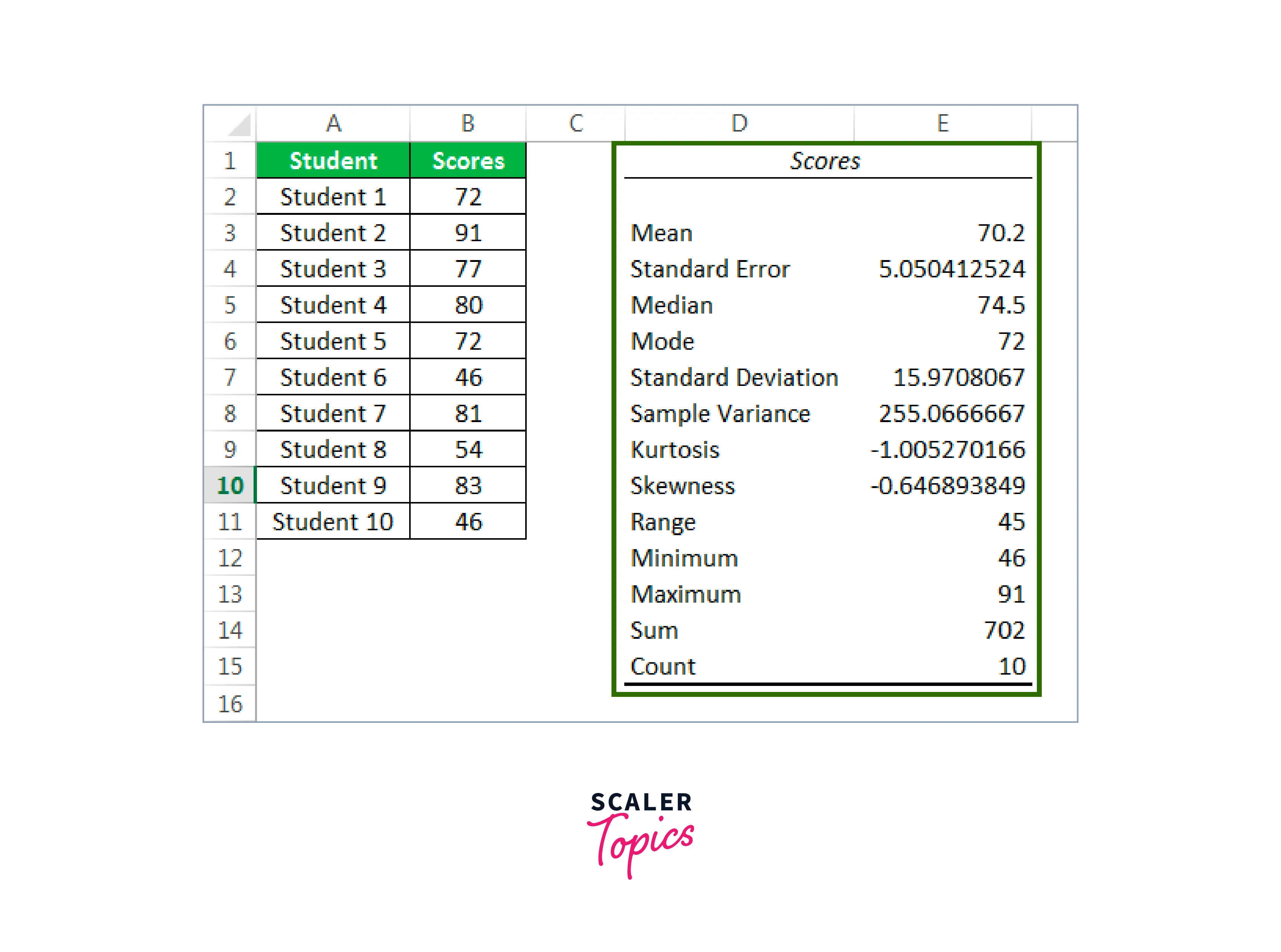
From the chosen data, we obtained various statistical findings or scores.

The standard deviation is 15.97, and the mean score is 70.2. Also, a 46 is the required minimum. At the same time, 91 is the highest possible score. Thus, the total score is 702, with 10 students in this sample. We have a variety of statistical findings in this manner.

Example 2

In the previous example, we learned how descriptive statistics operate. To use this Excel workbook for descriptive statistics, download it.

We have a list of students and information on their age, gender, height, weight, number of study hours per week, and recent exam results for a select handful.

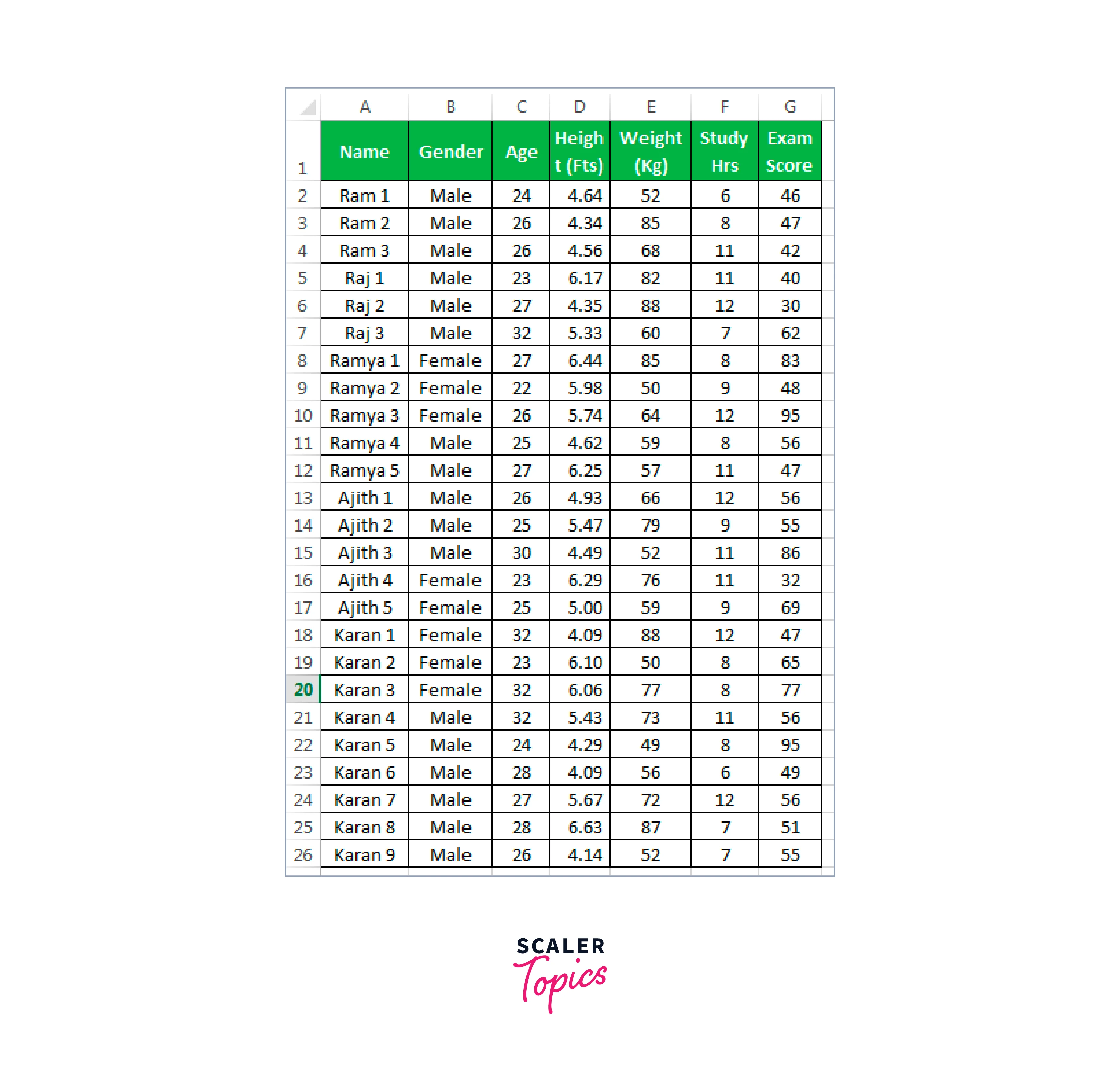
The following questions are frequently asked after looking at the data above: What is the average age of the student group? Average exam score, height, maximum value for each category, average weight, Minimum amount, etc.

Five alternative categories are available for us to use when presenting the statistical findings. So that we can discover all of these, we can perform a descriptive statistical study.

Step 1:
We must go to Data → Data Analysis.

Step 2:
By selecting "Data Analysis," we are presented with a list of all the available analysis methods. Scroll down after that and choose "Descriptive Statistics."

Step 3:
Select all category ranges, including the heads, under "Input Range," i.e., C1.

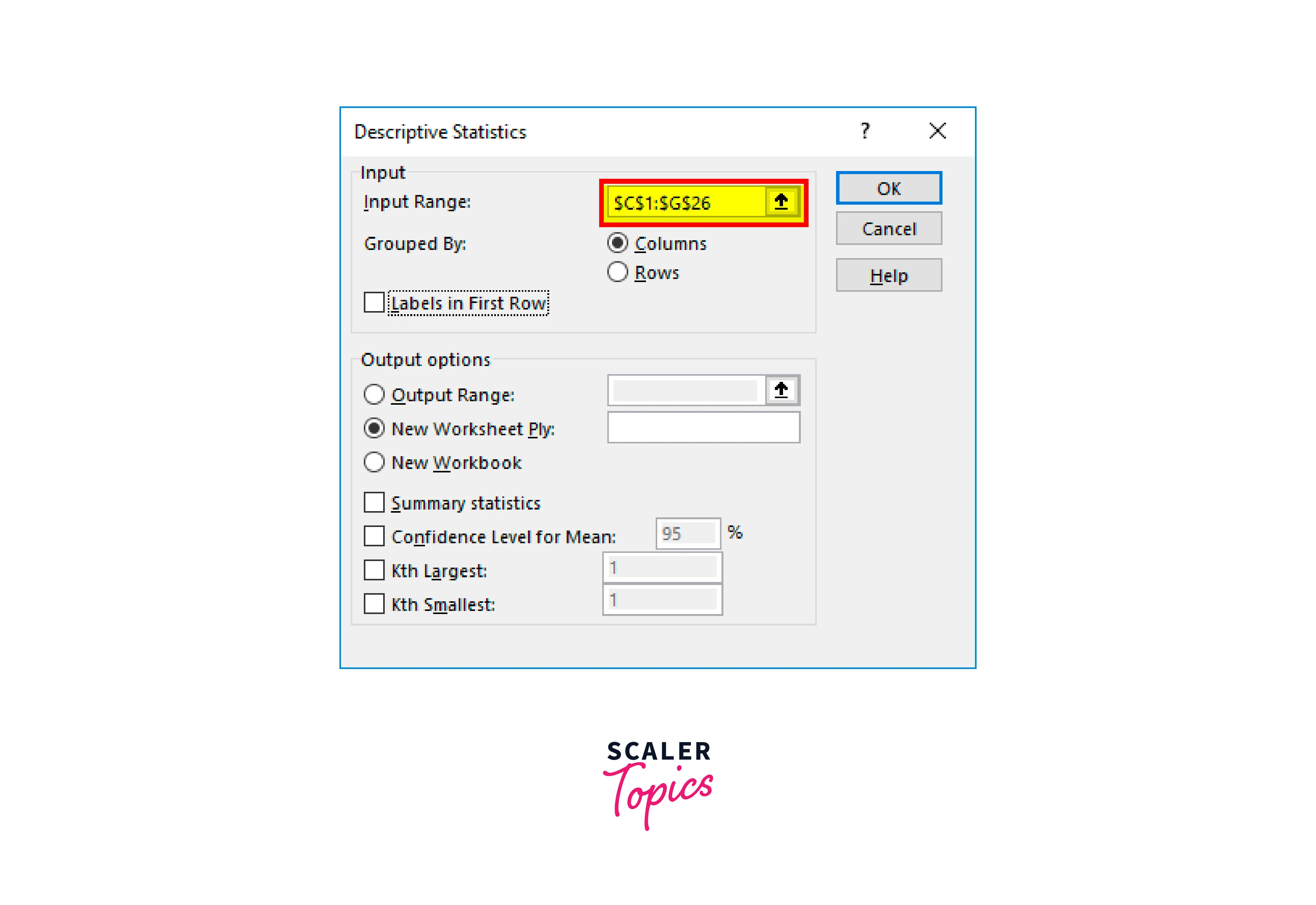
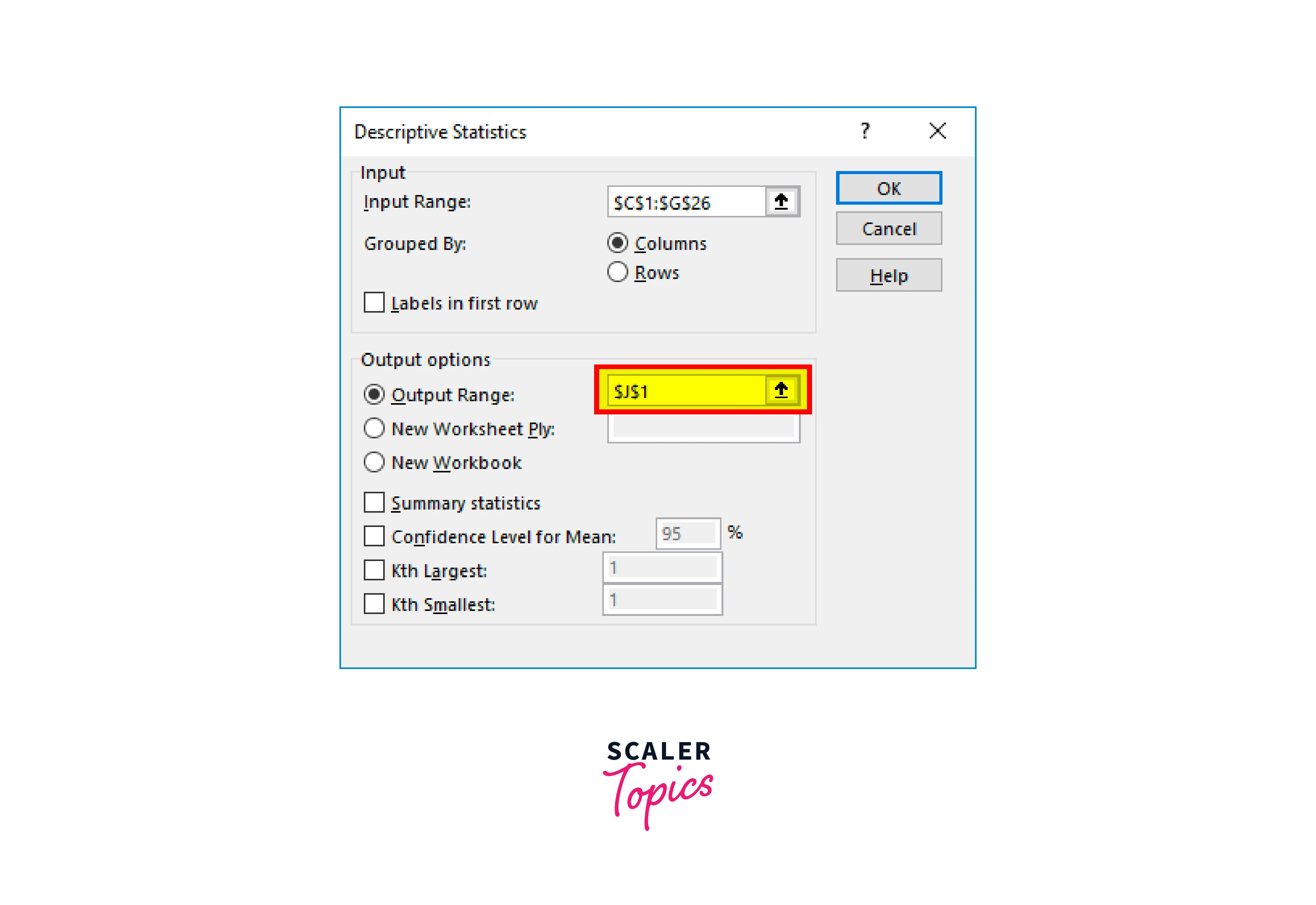
The summary result can be obtained in a workbook, a worksheet, or multiple worksheets. The summary report will then be displayed based on our choice. On the same worksheet, starting in the J1 cell, we have shown how to summarize.

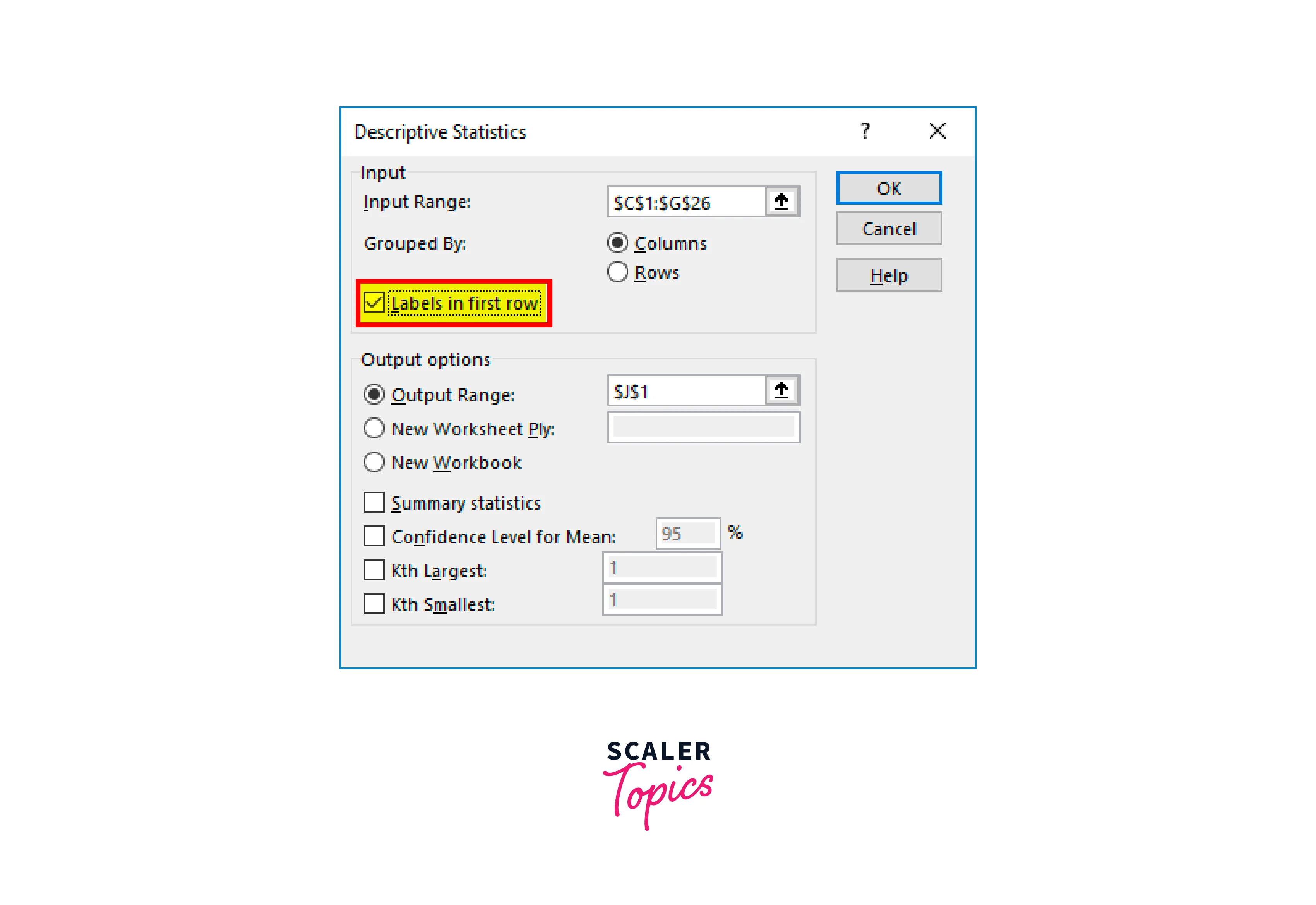
Considering that we have already chosen the headers, we must select "Labels in the first row." It will be useful for displaying the results because we have picked the headers. Otherwise, it would be difficult to grasp the results for each category.

Then select Summary Statistics from the menu.

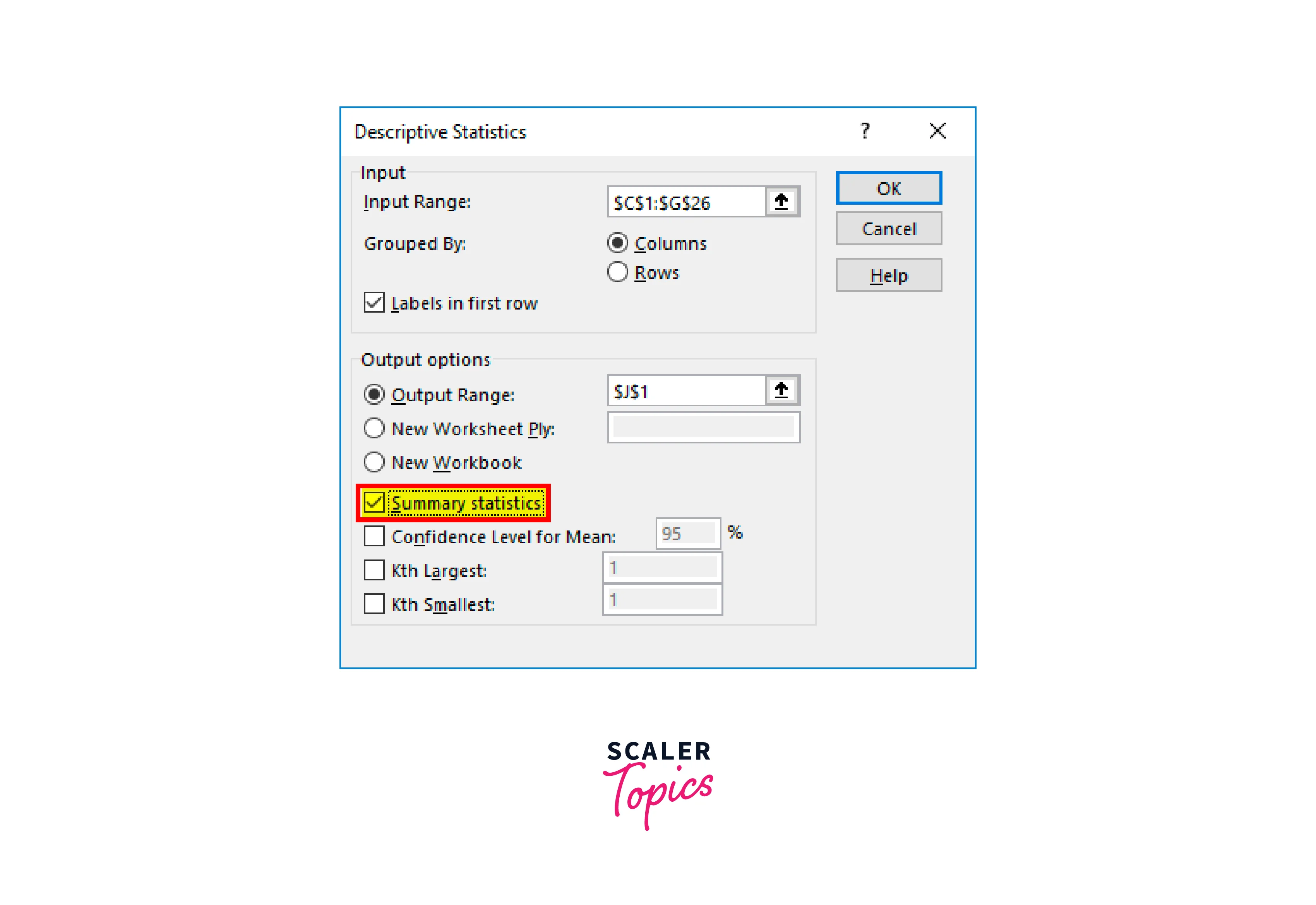
Step 4:
To finish the test, click "OK" after that. The J1 cell will provide us with the descriptive statistics findings.

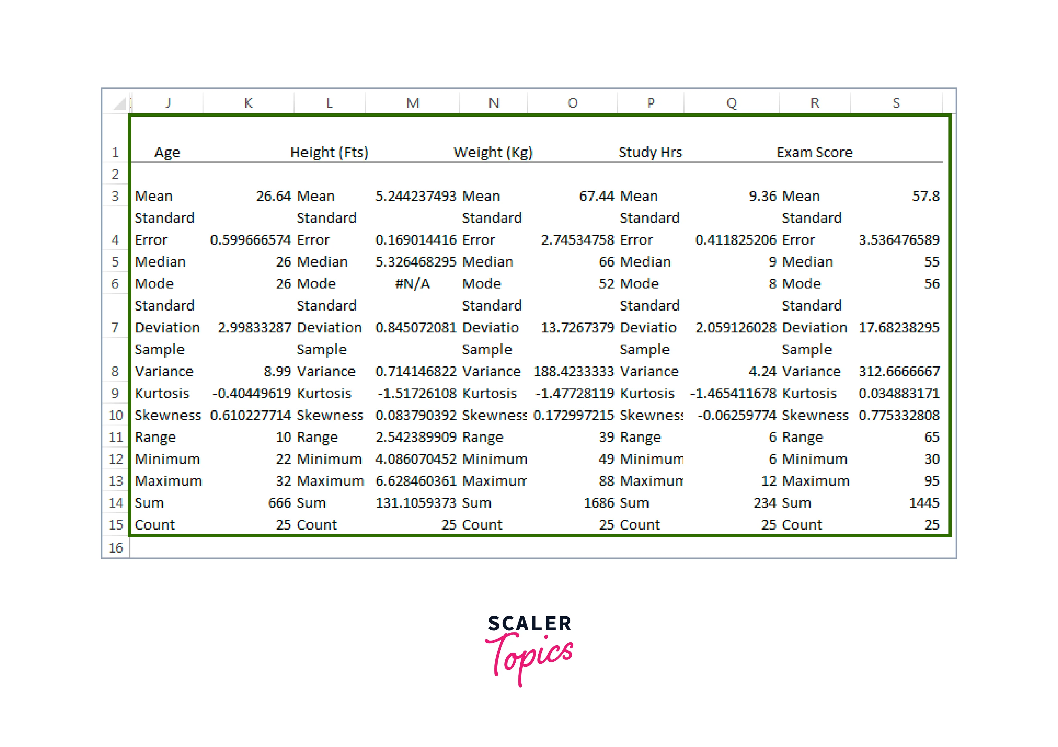
The statistical findings for each of the five categories have been displayed. Thus, for instance, the overall student population is 25, the average age is 26.64, the average height is 5.244, the average weight is 67.44, and the average exam score is 57.8, which is relatively low in comparison to today's standards and many other results.