Differences Between Discriminative and Generative Models

Overview

Machine learning models can be broadly classified into Discriminative and Generative. Discriminative models learn to model boundaries around classes in a dataset and estimate the conditional probability of the target variable given the data. Generative models, on the other hand, create new data points by estimating the joint probability distribution of the data and the target variable. Generative models are commonly used for unsupervised tasks, while discriminative models are often used for classification and Regression.

Introduction

Various Machine Learning models have been proposed over the years, each for different tasks. A broad categorization of these models is to classify them into Generative and Discriminative models.

Discriminative models estimate the conditional probability, while Generative models estimate the joint probability distribution. This article will examine the difference between Generative and Discriminative models. We will also introduce several commonly used ML models and categorize them into these two groups.

Discriminative Model

Discriminative Models are a family of models that do not generate new data points but learn to model boundaries around classes in a dataset instead. These models aim to maximize the separation between the classes in the dataset to perform classification or Regression. Discriminative models estimate the conditional probability $P(Y|X =x)$ on a data X and a target Y.

Note: that sometimes classifiers that do not use a probability model are called Discriminative Models.

Logistic Regression

Logistic Regression is a classification algorithm that uses the Sigmoid function instead of a linear function to model data.

The Sigmoid curve is shown in the figure below.

sigmoid-curve-dl

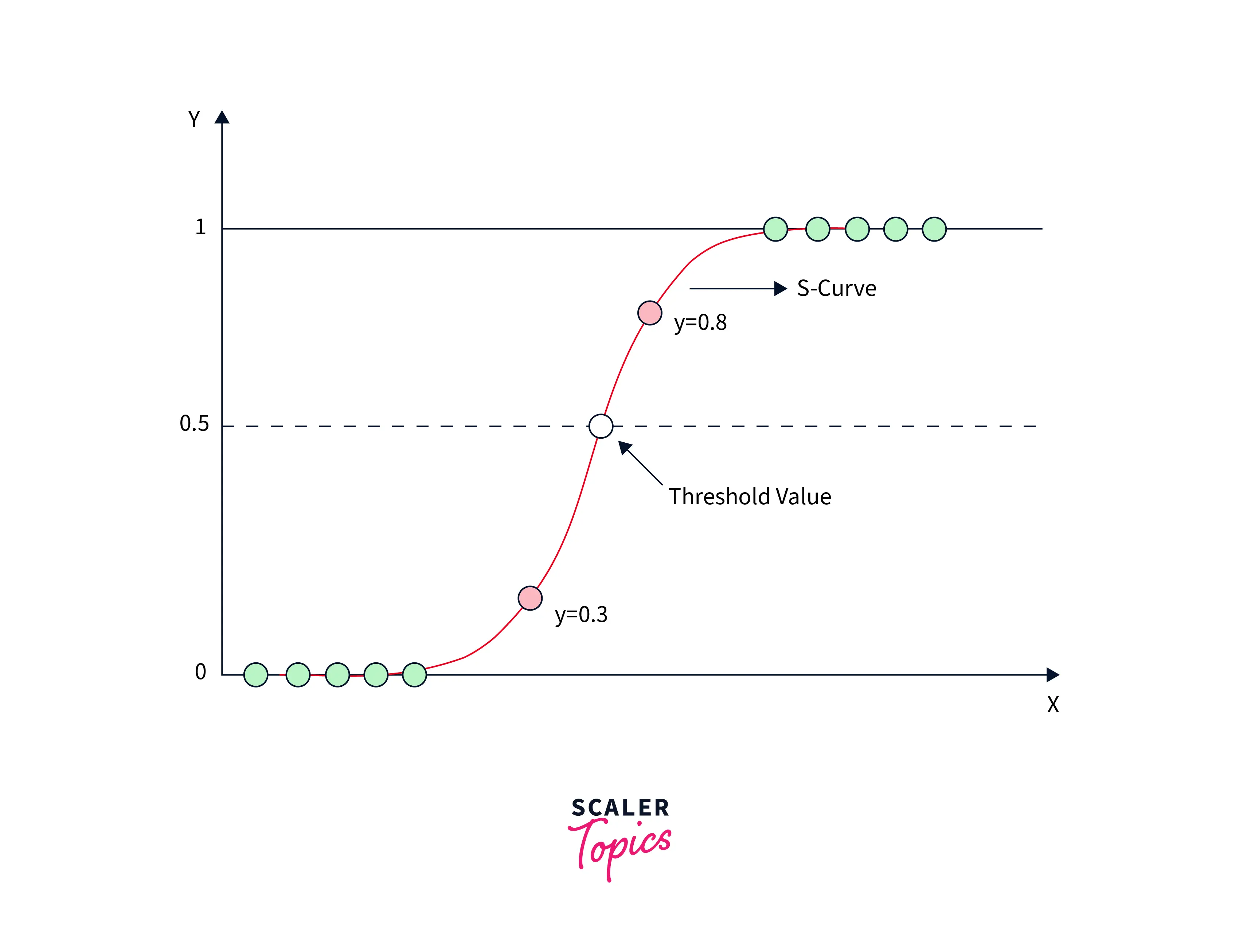
We can also use Logistic Regression for multi-class tasks by modeling each class separately. Therefore, the Regression's outcome must be a discrete or categorical value. (e.g., Yes/No, True/False) The model's output is a probabilistic value in the range $[0,1]$ . The modeled curve that the logistic function uses indicates the likelihood of the binary decision. The following equation can mathematically represent Logistic Regression.

$log[\frac{y}{1-y}] = b_0 + b_1 x_1 + b_2 x_2 + … + b_n x_n$

Considering the difference between Generative and Discriminative models is important in understanding why these models are Discriminative.

Support Vector Machine

A Support Vector Machine (SVM) is a supervised classification and regression algorithm that uses the concept of hyperplanes. These hyperplanes can be understood as multi-dimensional linear decision boundaries that separate groups of unequal data points. An example of a hyperplane is shown below.

svm-in-dl

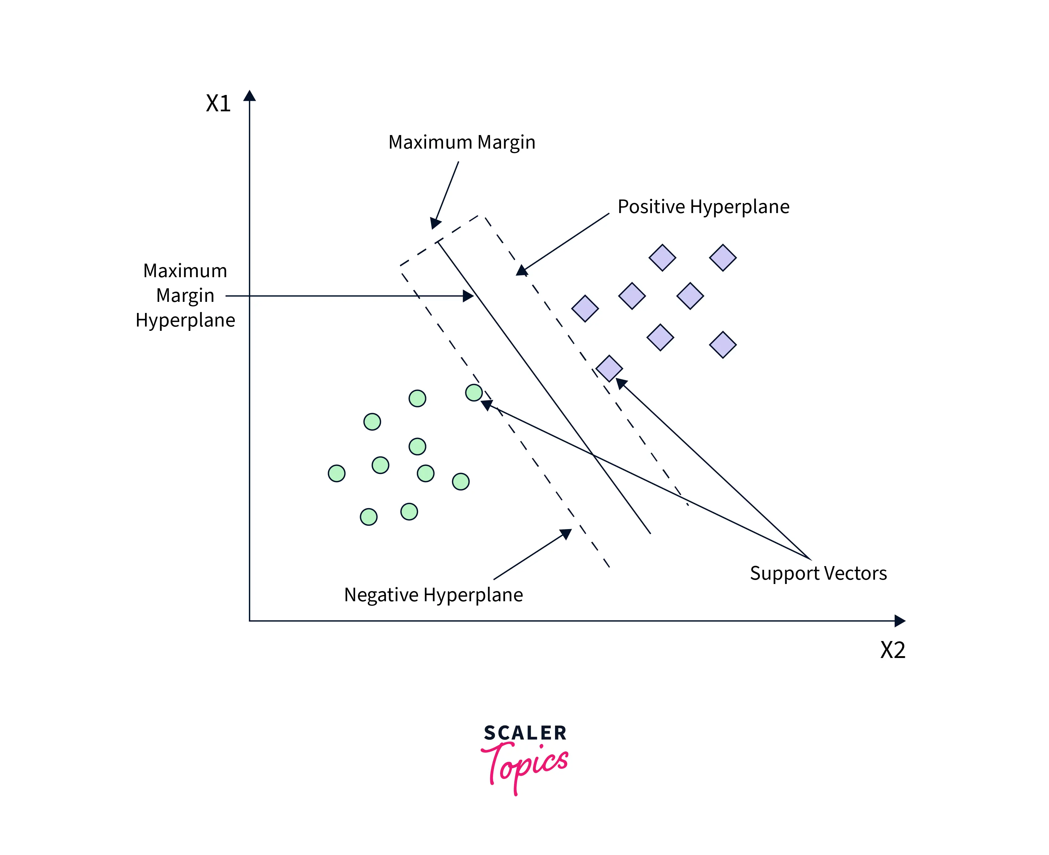
An optimal fit of the SVM occurs when a hyperplane is furthest from the training data points of any of the classes—the larger this distance margin, the lower the classifier's error.

To better understand how the SVM works, consider a group of data points like the one shown in the diagram. It is a good fit if the hyperplane separates the points in the space, so they are clustered according to their labels. If not, further iterations of the algorithm are performed.

Decision Tree

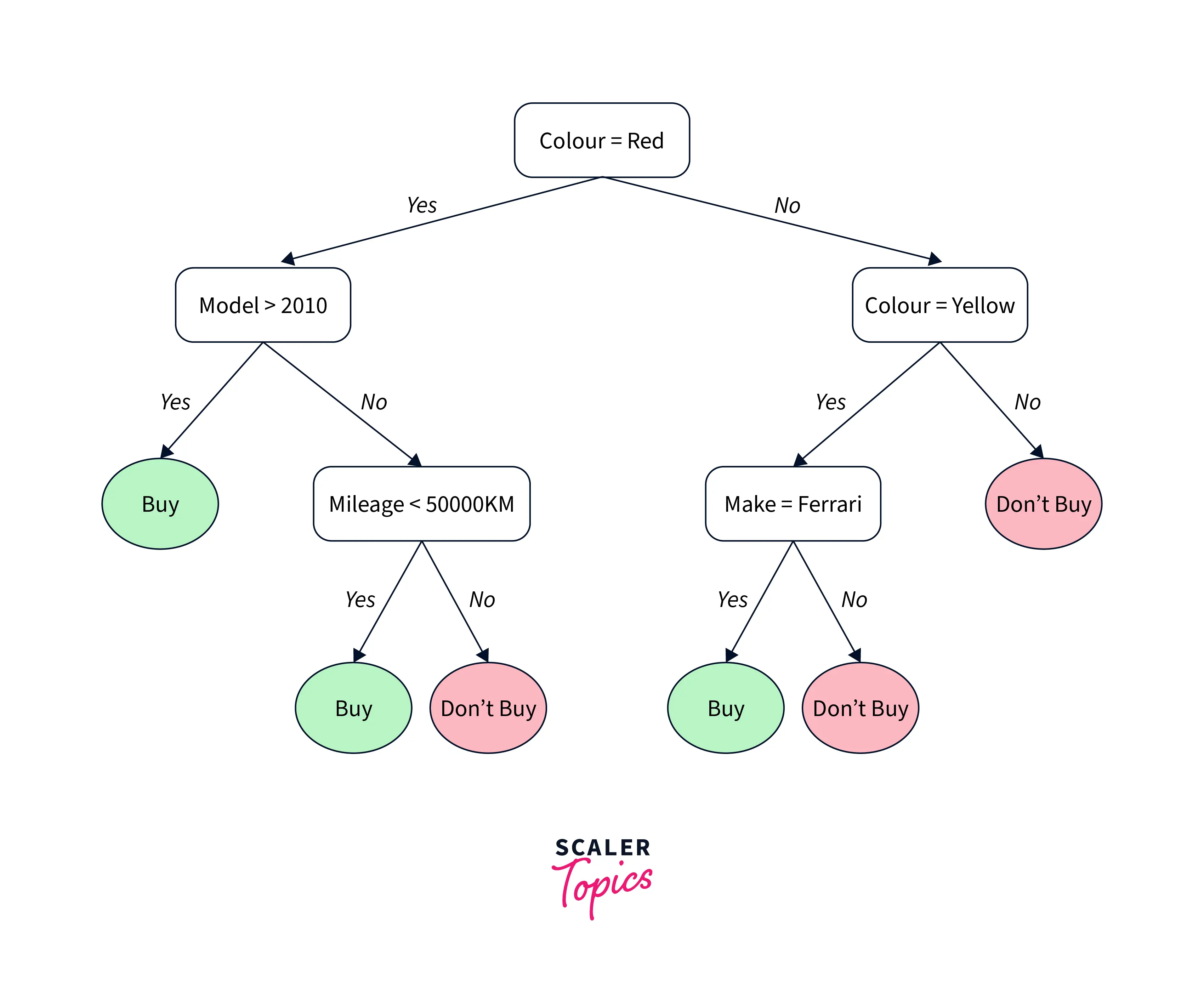
Decision trees are tree-based decision models that use a root node internal structure followed by successive child leaf nodes. The leaf nodes are a placeholder for the classification label, and the branches show the outcomes of the decision. The paths from the tree's root to the leaves represent the classifier rules. Each tree and sub-tree models a single decision and enumerates all the possible decisions to choose the best one. A Decision tree can be optimal if it represents most of the data with the least number of levels.

Decision trees are helpful for classification but can be extended for Regression using different algorithms. These trees are computationally efficient, and many tree-based optimizations have been created over the years to make them perform even faster.

An example of such a tree is shown below. decision-tree

Random Forest

random-forest

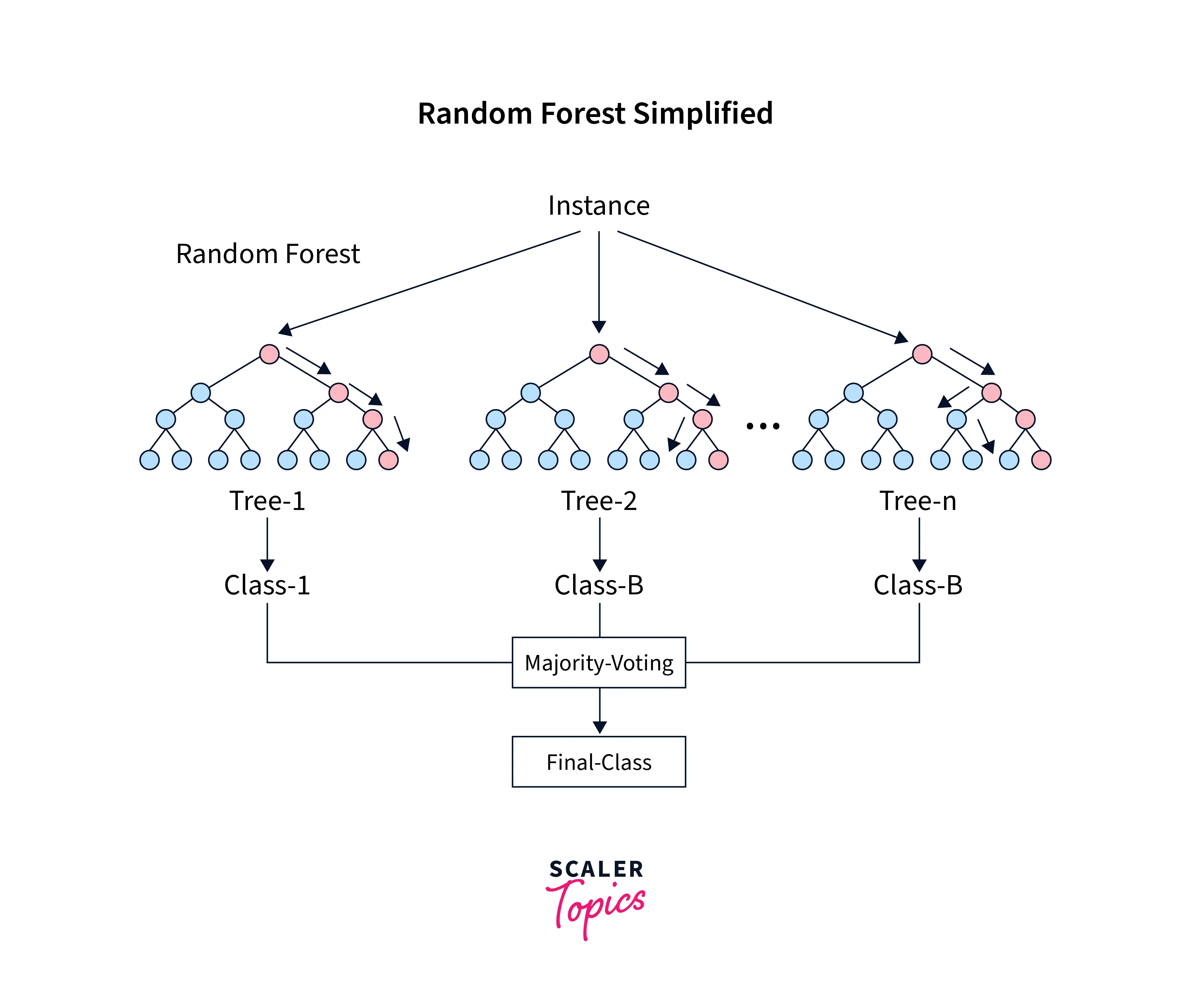
Random Forest models use a forest of Decision Trees to make better decisions by combining each tree's decisions. The most popular decision across the trees for a task is the best after the aggregation. This technique of aggregating multiple results from similar processes is called Ensembling.

The second component of the Random Forest pertains to another technique called Bagging. Bagging differs from Ensembling because, in Bagging, the data is different for every model, while in Ensembling, the different models are run on the same data.

In Bagging, a random sample with replacement is chosen multiple times to create a data sample. These data samples are then used to train the model independently. After training all these models, the majority vote is taken to find a better data estimate.

Random forests combine the concepts of Bagging and Ensembling to decide the best feature splits and select subsets of the same. This algorithm is better than a single Decision Tree as it reduces bias and the net variance, generating better predictions.

Bagging and Ensembling might seem like they help model the joint probability distribution, but that is not the case. Understanding the difference between Generative and Discriminative models can clear this confusion.

Generative Models

Generative Models are a family of models that create new data points. They are generally used for unsupervised tasks. Generative Models use the joint probability distribution $P(X, Y)$ on a variable X and a target variable Y to model the data and perform inference by estimating the probability of the new data point belonging to any given class.

Latent Dirichlet Allocation (LDA)

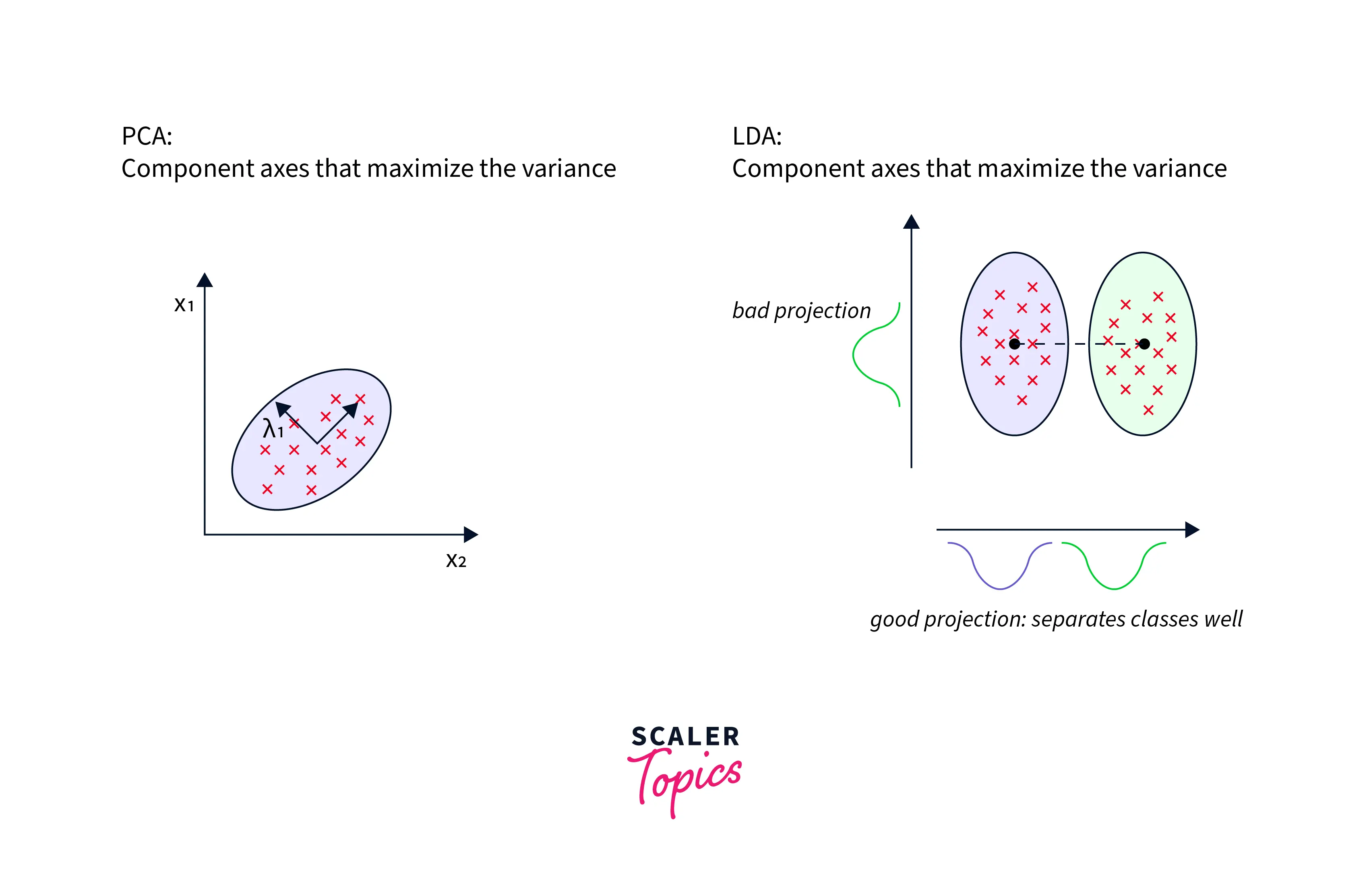
LDA models aim to accurately estimate the classwise mean and variance of the data points in a given dataset. After calculating these statistics, LDA makes predictions by estimating the probability of the new class belonging to any classes in the original data. In ML, LDA models are used for topic modeling and discovery. LDA is similar to PCA in that it also performs a dimensionality reduction. But unlike PCA, LDA maximizes the class separation and not the variance of the data.

This principle is illustrated in the figure below.

lda-in-dl

Bayesian Network

A Bayesian Network is a graph-based probabilistic model that uses a special graph structure known as a DAG - Directed Acyclic Graph to model conditional dependencies between the given variables. Given several contributing factors, these networks are useful in finding the possible cause of an event.

A classic example of what a Bayesian Network looks like is shown below.

bayesian-network-in-dl

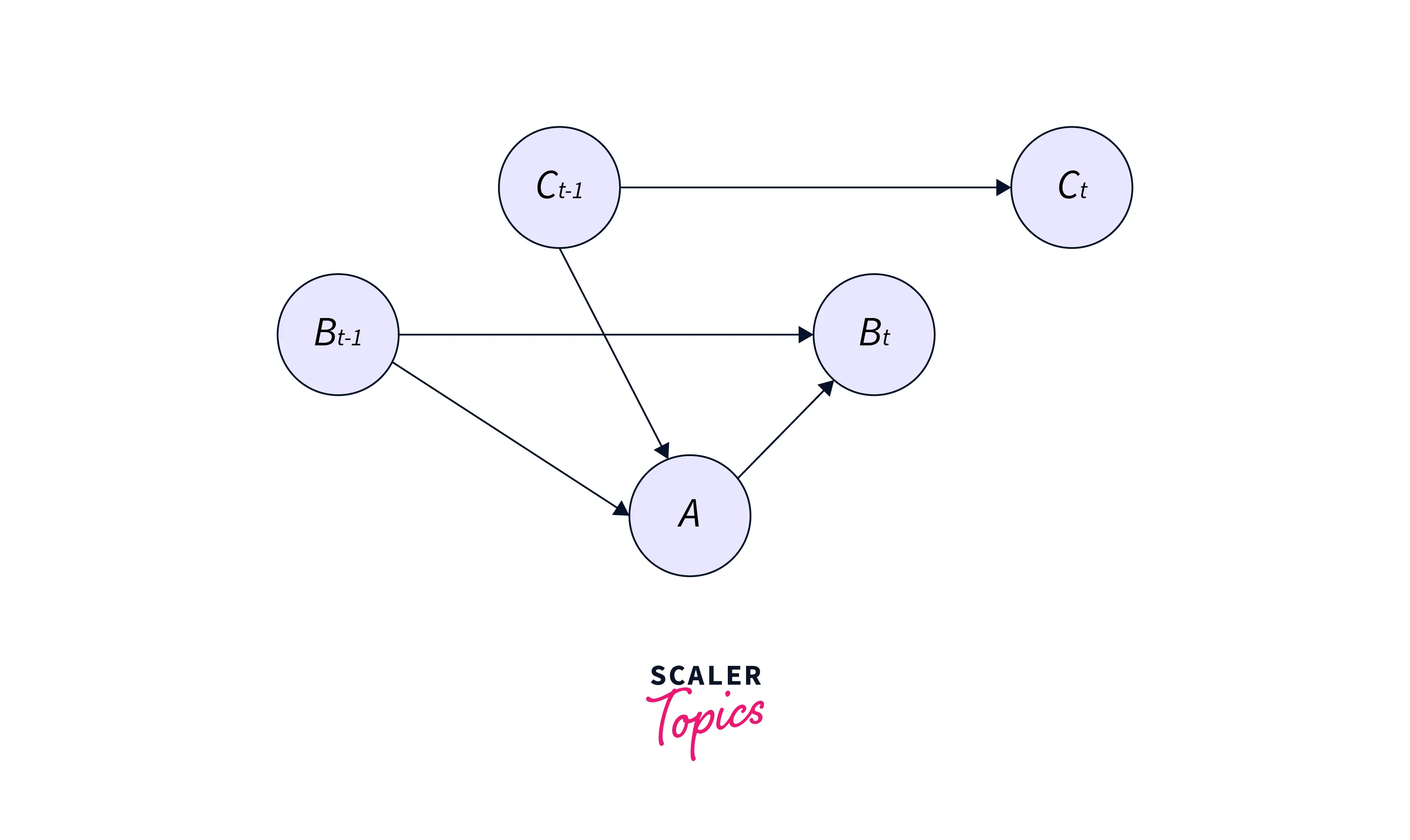
The Bayesian Network uses this graph to model the joint probability distribution. Each of the edges in the graph represents a dependency, while each node represents a unique variable. The model can then use this learned distribution for inference.

We can use Bayesian Networks to infer unobserved variables, learn parameters from the data and learn the structure of a manually created data distribution.

Note: that each represents Boolean variables if there are $m$ parent nodes. A minimum of $2^m$ entries are required to model the possible events.

Hidden Markov Model

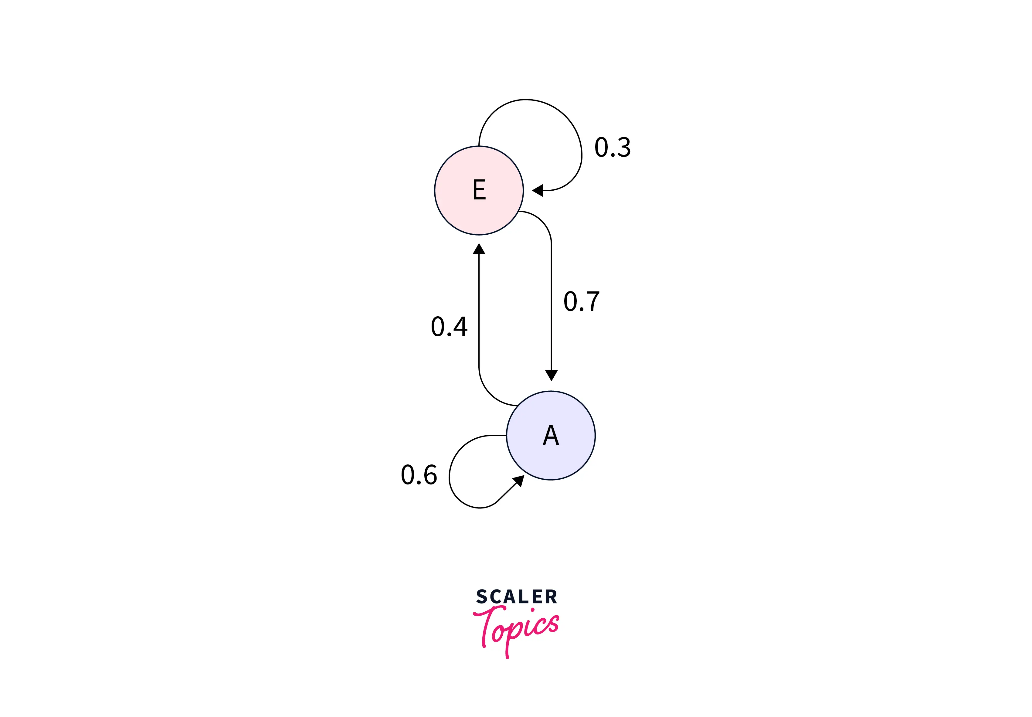
A Markov process is a sequential process where the previous item only influences the next item in the sequence. A Markov Chain, therefore, is a graph that uses probabilities to denote how likely it is to move to the next stage in the chain. (If it is not clear how this is a Generative model, refer to the section on the difference between Generative and Discriminative models)

An example Markov Chain is shown below. markov-chain-in-dl

A Hidden Markov Model is a graph where the chain is unobservable. The inputs the model receives are combined with the probabilities of the previous step. This combination is used to calculate the next step in the graph.

A constraint in an HMM is that at a certain time $t= t_{0}$ , the target Y must be influenced only by the state of X at $t= t_{0}$ . The states of Y at $t= t_{0}$ should not be affected by the states of X and Y at $t < t_{0}$ .

An example of a Markov Model is shown here for reference. hmm-in-dl

Autoregressive Model

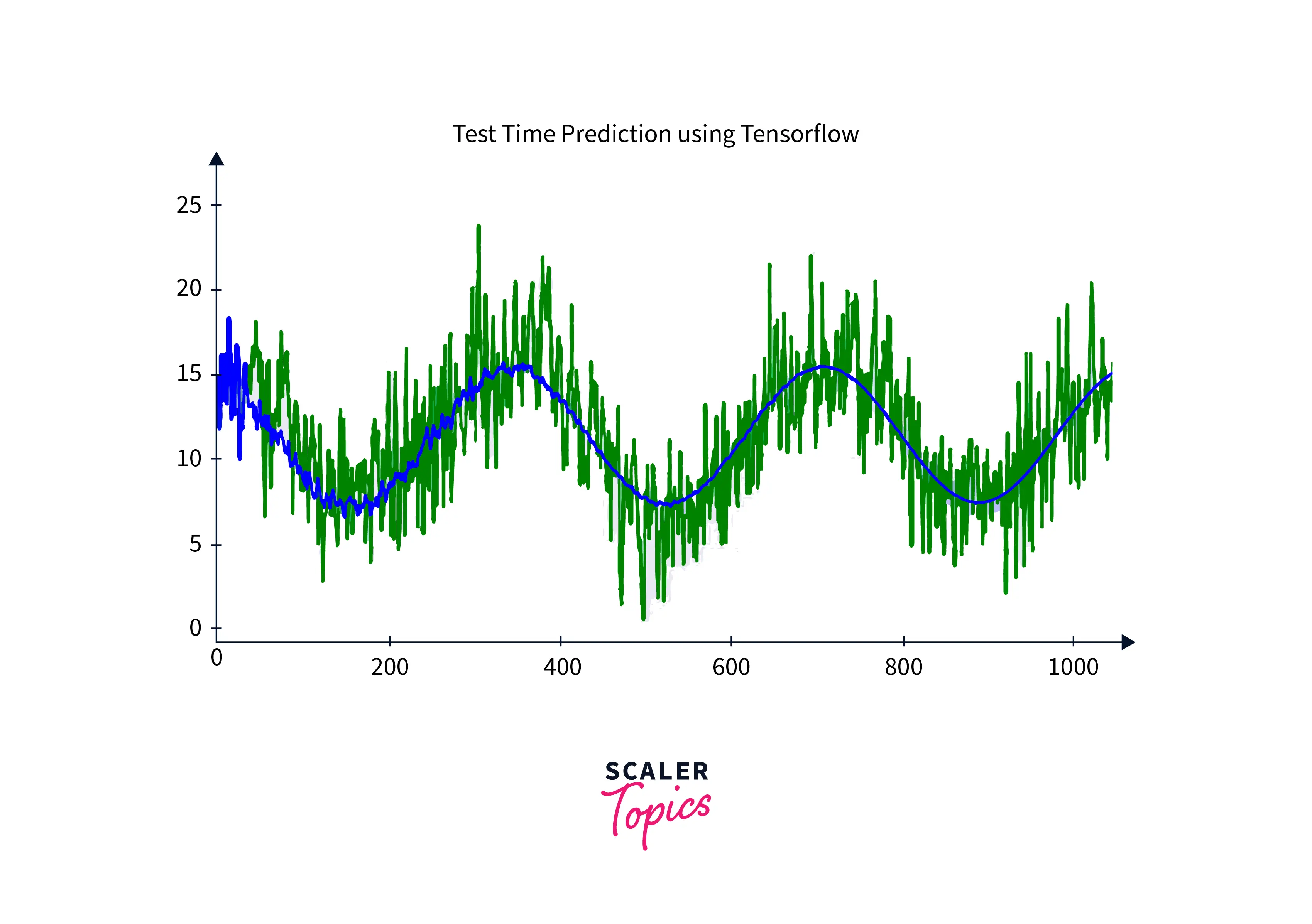
An Autoregressive model is used in time series forecasting. This model uses the past values in the time series to predict values that might occur in the future.

An Autoregressive model gets its name as it is a regression of itself. These models are generally represented as stochastic difference equations that use linear combinations of past values to model the data. A mathematical representation is as follows.

$y_{t} + c + \phi_{1} y_{t-1} + \phi_{2} y_{t-2} + … + \phi_{p} y_{t-p} + \epsilon_{t}$

where $\epsilon_{t}$ is white noise.

Note: that changing the patterns for $\phi$ changes the time series. Varying the error term does not change the pattern but modifies the scale of the data instead.

An example of an Autoregressive model is shown below. autoregressive-model-in-dl

Generative Adversarial Network

Generative Adversarial Networks are models that take large image datasets as input and generate new images. A GAN models the data distribution by exploiting the latent space of the given dataset.

A GAN comprises two parts - A Generator and a Discriminator. These parts play a MinMax Game, where the Generator creates novel images from random noise while the Discriminator classifies the outputs into real or fake. When the Discriminator can no longer distinguish between real and fake images created by the Generator, the GAN training is said to be complete.

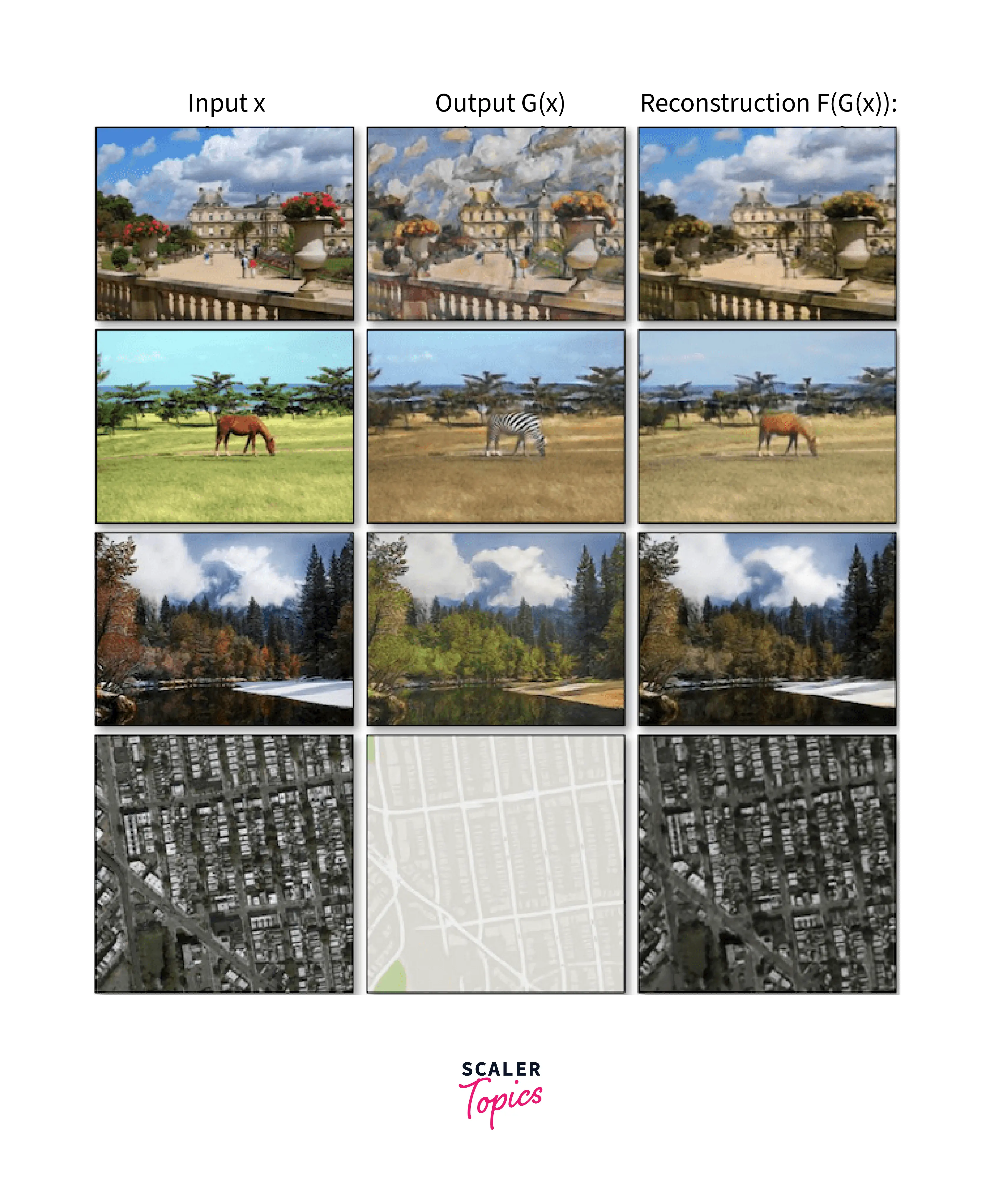
An example of a GAN that converts images to a different style is shown in the following image.

gan-in-dl

Discriminative vs. Generative Models

Generative models are a class of machine learning models that aim to understand the underlying probability distribution of the data. They try to learn the underlying structure of the data by modeling the joint probability of the inputs and outputs. A common example of a generative model is a Gaussian Mixture Model (GMM), which models the data as a collection of Gaussian distributions. These models can be used for unsupervised tasks like anomaly detection, density estimation, and generative art.

Discriminative models, on the other hand, aim to model the decision boundary between different data classes. They try to learn the boundary between different data classes by modeling the conditional probability of the outputs given the inputs. A common example of a discriminative model is a Support Vector Machine (SVM) which models the data as a boundary that maximally separates different classes. These models can be used for supervised tasks like classification and Regression.

Generative models thus try to understand the underlying probability distribution of the data, while Discriminative models try to model the decision boundary between different data classes. Generative models are computationally more expensive and susceptible to outliers but can be used for unsupervised tasks. Discriminative models are computationally cheaper and are more robust to outliers but are mainly used for supervised tasks.

The difference between the Generative and Discriminative models is summarised in the following table.

Generative Models	Discriminative Models
Aim to understand the data distribution.	Aim to model the data decision boundary.
Uses the joint probability.	Uses conditional probability.
Relatively computationally expensive.	Relatively cheaper computationally.
Unsupervised Tasks.	Supervised Tasks.
Harmed by outliers.	More robust to the presence of outliers.
Models how data is placed in space.	Generates boundaries around similar classes of data in space.

Conclusion

In summary, discriminative and generative models are two machine learning models that approach tasks differently.
Discriminative models aim to maximize the separation between classes in a dataset to perform classification or Regression.
In contrast, generative models create new data points by estimating the data's and target variable's joint probability distribution.
Both models have their own set of advantages and disadvantages and can be applied to various tasks.

Differences between Discriminative and Generative Models

Overview

Introduction

Discriminative Model

Logistic Regression

Support Vector Machine

Decision Tree

Random Forest

Generative Models

Latent Dirichlet Allocation (LDA)

Bayesian Network

Hidden Markov Model

Autoregressive Model

Generative Adversarial Network

Discriminative vs. Generative Models

Conclusion