Basic Excel Formulas

Using Excel Formulas

1. Create a Excel Formulas that Refers to Values in Other Cells

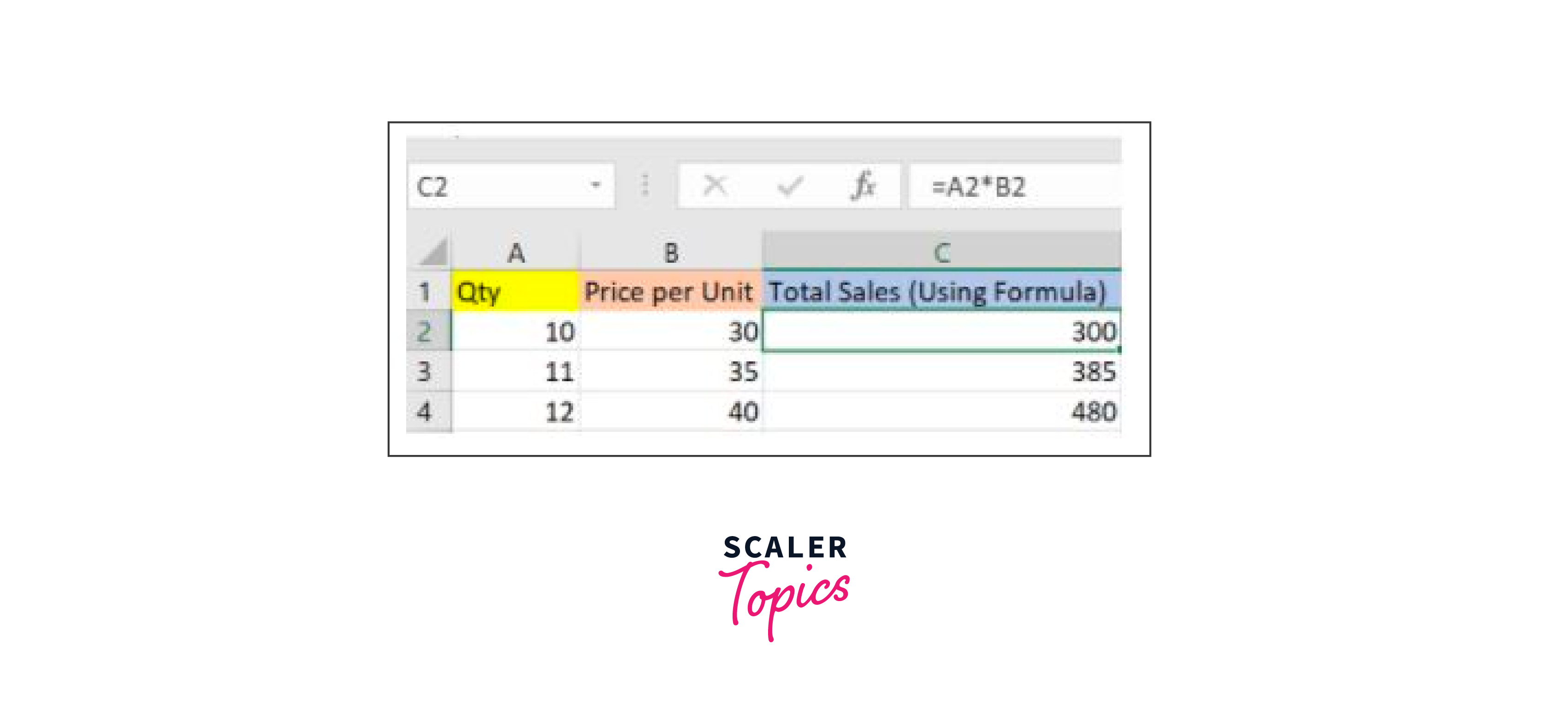
The following example shows how we manually applied the multiplication formula with the '*' operator.

Sample Formula: "=A2*B2"

2. See a Formula

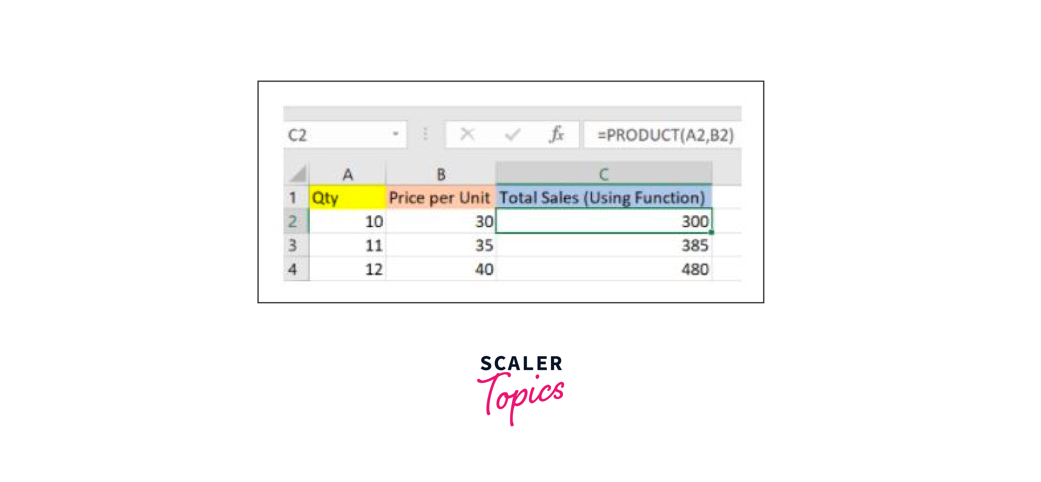
The example below shows how we performed multiplication using the function 'PRODUCT'. As you can see, we removed the mathematical operator from this situation.

3. Enter a formula that contains a built-in function

Sample Formula: "=PRODUCT(A2,B2)"

Excel functions and Excel Formulas save you time and help you complete jobs effectively. Let's go on to learn the many functions that Excel offers and use the appropriate formulas as and when necessary.

Top Excel Formulas List with Examples

Depending on the type of operation you wish to carry out on the dataset, a variety of Excel Formulas and functions are available. We'll examine mathematical operation formulas and functions, character-text formulae, data and time formulas, sumif-countif formulas, and lookup Excel Formulas.

The top 25 Excel Formulas you need to know are now discussed. In this post, we've divided 25 Excel formulas into categories based on how they function. The first Excel Formulas on our list should be our first focus.

1. SUM

As its name implies, the SUM() function returns the sum of the values in the selected range of cells. It performs the addition mathematical operation. Here is an example of it:

Sample Formula: "=SUM(C2)"

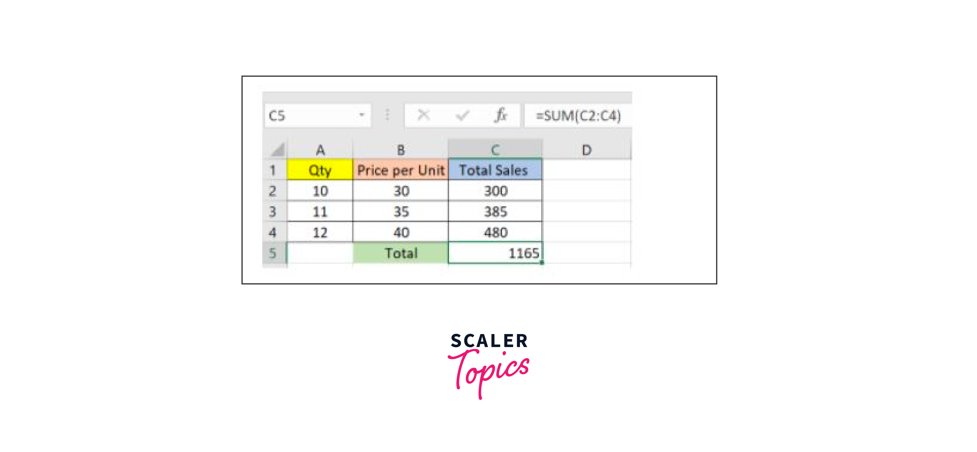
As you can see above, all we had to do was enter the function "=SUM(C2)" to determine the total amount of sales for each unit. The sum of these three numbers is 300, 385, and 480. The outcome is kept in C5.

2. AVERAGE

The AVERAGE() function aims to determine the average value across the chosen range of cell values. As seen by the example below, you need only type the following to determine the average of all sales:

=AVERAGE(C2, C3, C4)

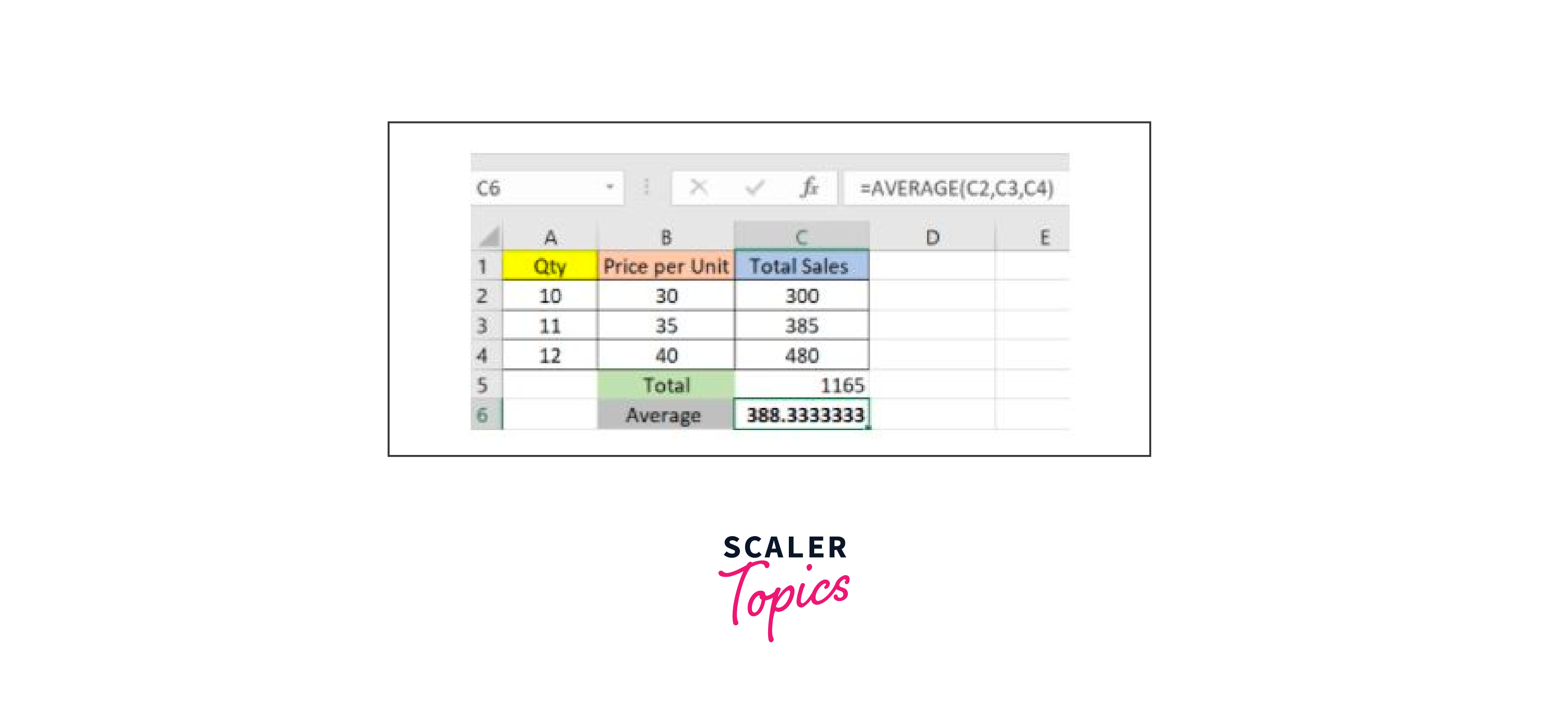
The average is computed automatically; you can store the outcome wherever you like.

3. COUNT

The COUNT() function counts every cell in a range of cells that contain a number. It excludes the empty cells and those that contain information in a format other than numeric.

Sample Formula: "=COUNT(C1)"

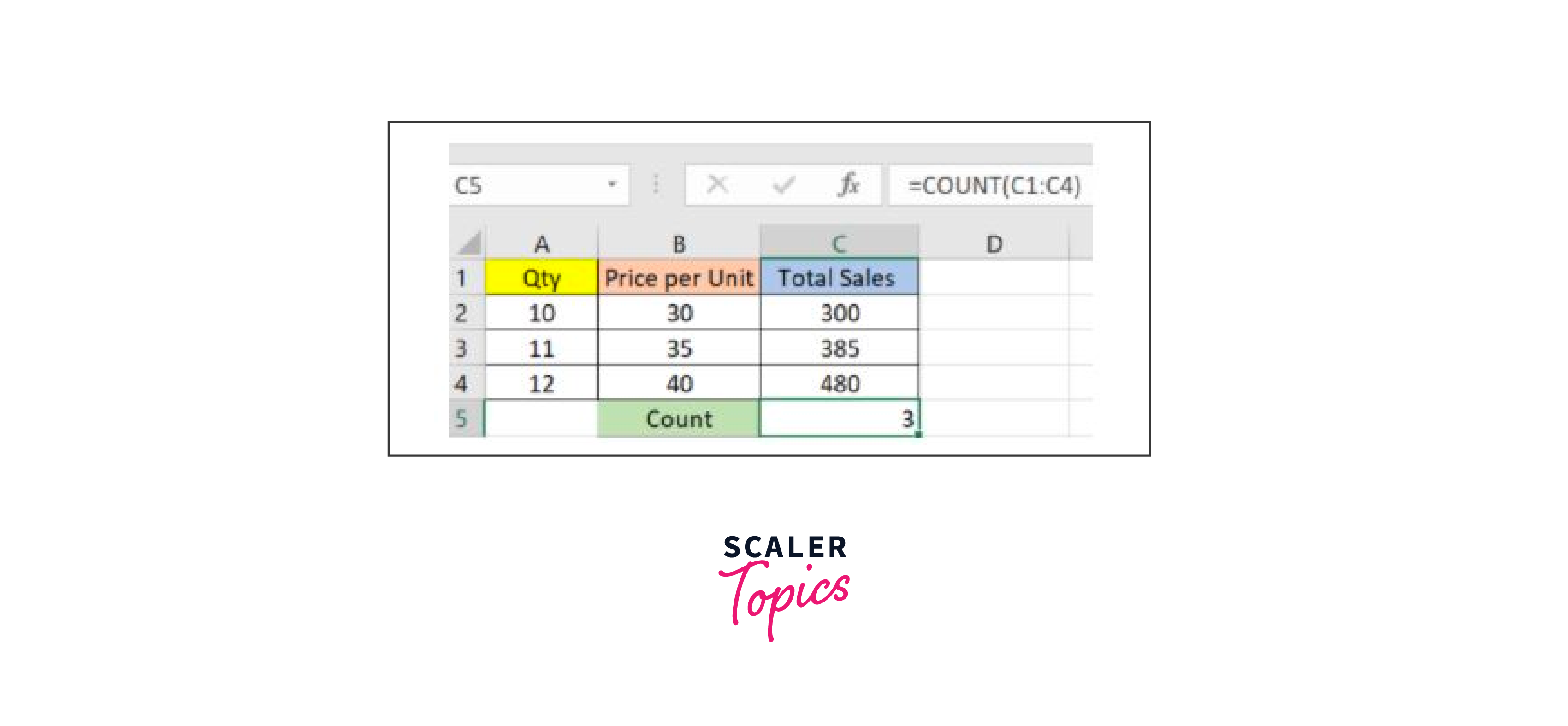
As seen above, we are counting from C1 to C4, the ideal number of cells. However, because the COUNT function only considers cells with numerical values, the correct response is 3, since the "Total Sales" cell has been left out.

Use the function "COUNTA()" if you need to count all the cells containing text, numeric values, or any other data type. However, blank cells are not counted by COUNTA().

COUNTBLANK() is used to count the number of blank cells in a range of cells.

4. SUBTOTAL

Let's proceed to understand the subtotal function now. The subtotal in a database is returned by the SUBTOTAL() function. You can choose between average, count, sum, minimum, maximum, and other options based on your needs. Let's look at two such instances.

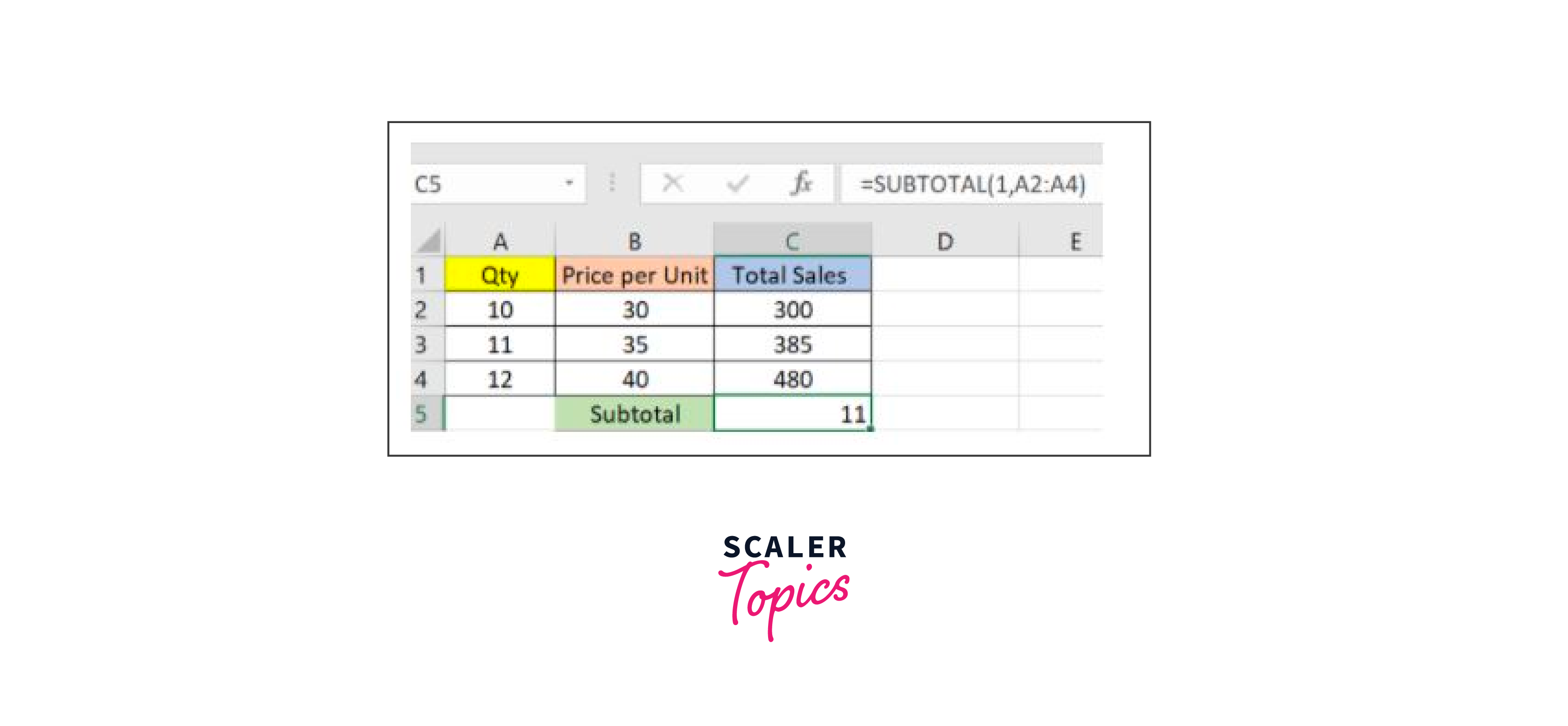
In the above example, cells A2 to A4 were used to calculate the subtotal. You can see that the function is

“=SUBTOTAL(1, A2: A4)"

The average is shown by "1" in the subtotal list. As a result, the previously mentioned approach will return A2's average as A4 and A2's response as 11, which is kept in C5. Similarly,

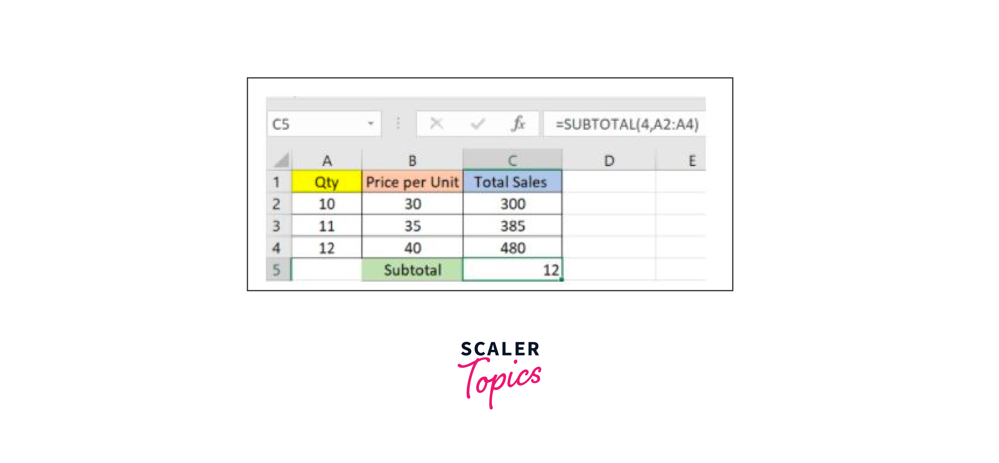
“=SUBTOTAL(4, A2: A4)” This chooses the cell from A2 through A4 with the highest value, which is 12. The maximum result is obtained when "4" is included in the function.

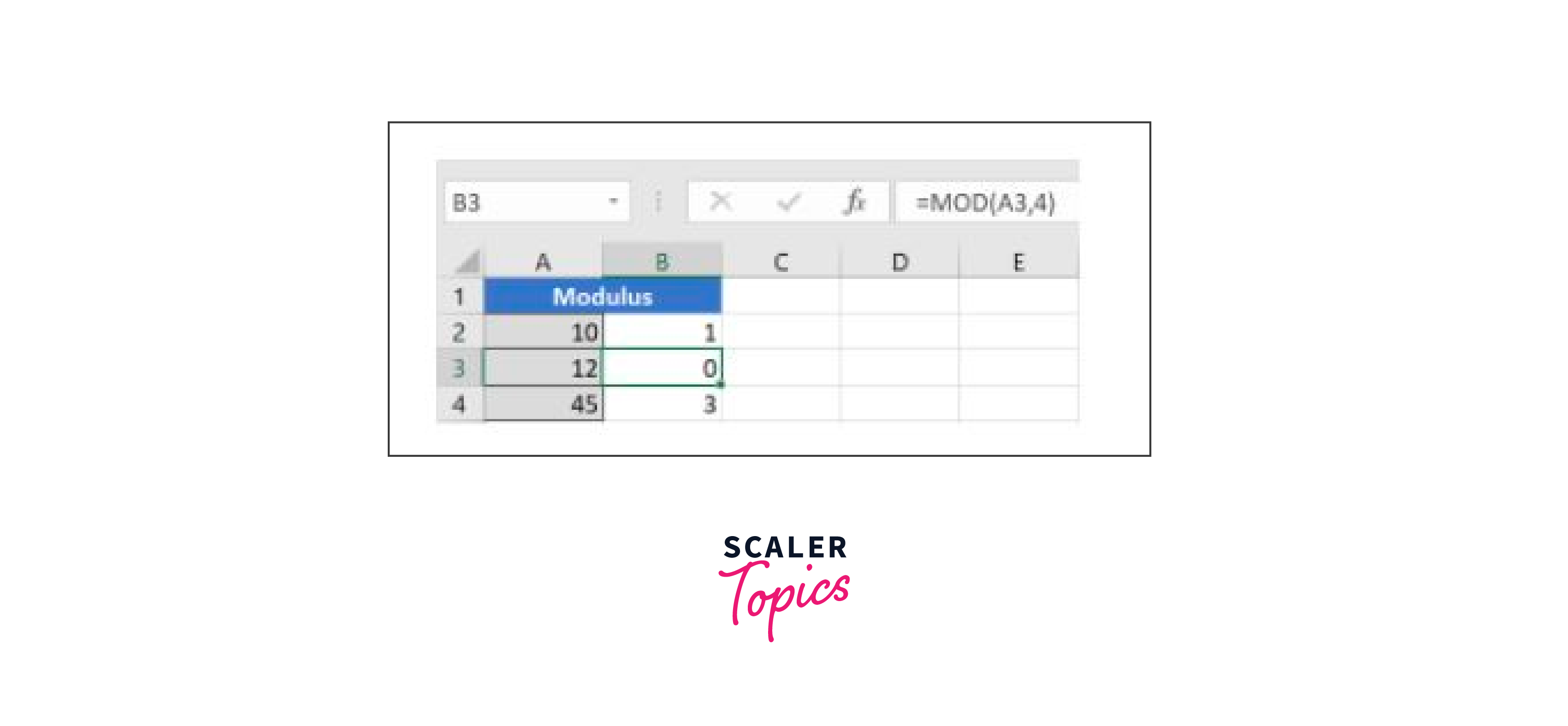
5. MODULUS

The MOD() Excel Formulas aims to return the remaining after dividing a given number by a divisor. For a better understanding, let's look at the samples below.

For the first example, we divided 10 by 3. The function is used to determine the remaining.

“=MOD(A2,3)”

The result is kept in B2. Alternatively, we can just type "=MOD(10,3)" and get the same result.

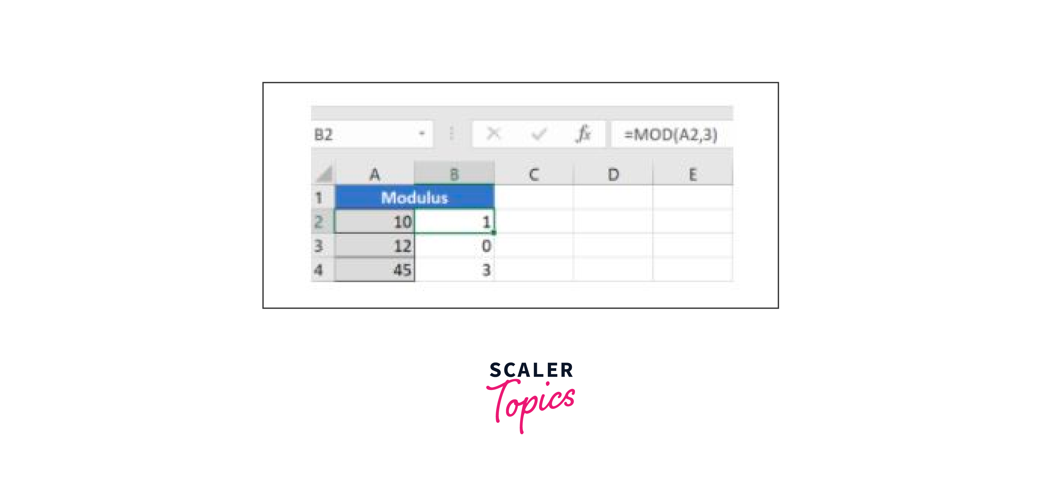
Likewise, we have divided 12 by 4 here. 0 is the remaining amount, and it is kept in B3.

6. POWER

The output of an integer raised to a specific power is returned by the method "Power()". Let's look at the following examples:

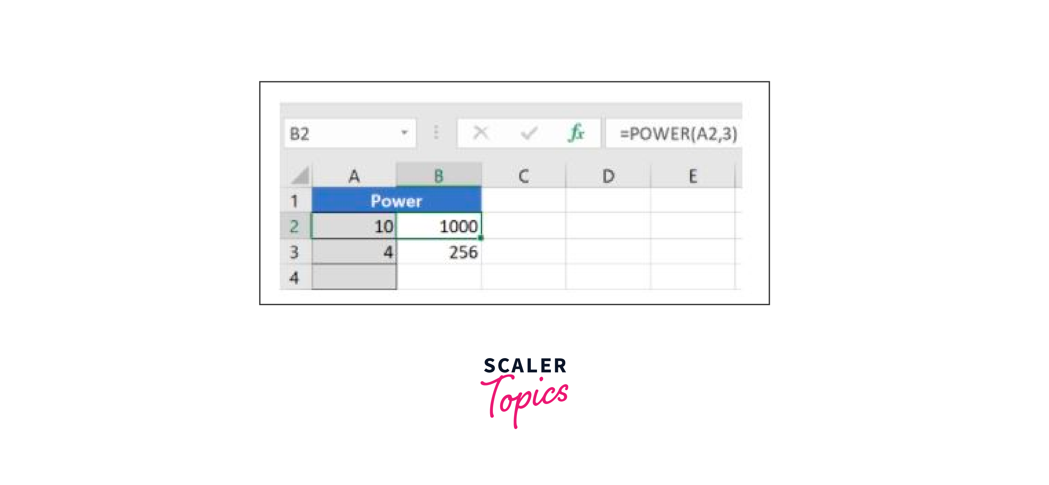
As you can see above, we must type: to find the power of 10 stored in A2 raised to 3.

“= POWER (A2,3)”

This is how Excel's power function operates.

7. CEILING

The ceiling function comes next. A number is rounded up to the nearest multiple of importance using the CEILING() function.

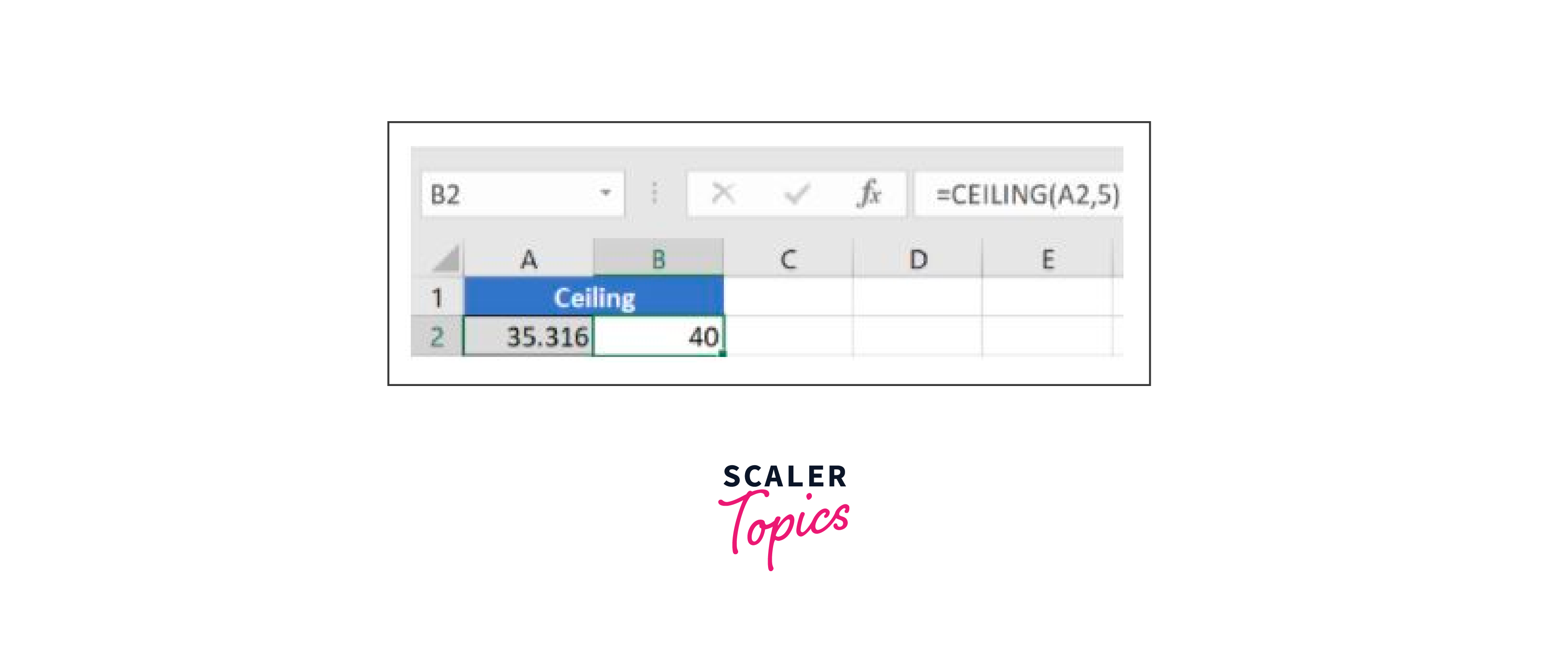
For 35.316, 40 is the biggest multiple of 5 close by.

8. FLOOR

The floor function reduces a number to the nearest multiple of importance, in contrast to the ceiling function.

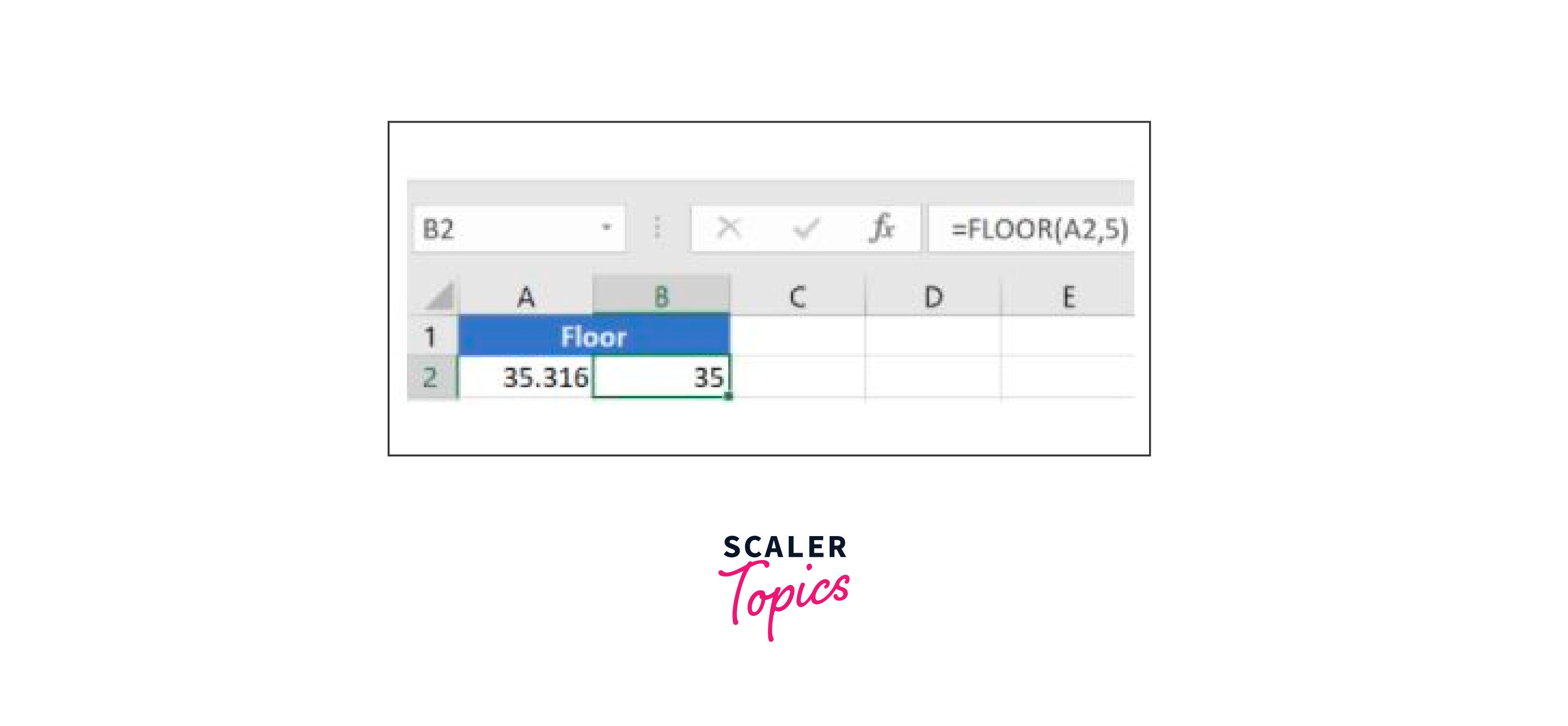
35 is the lowest multiple of 5, is close by for 35.316.

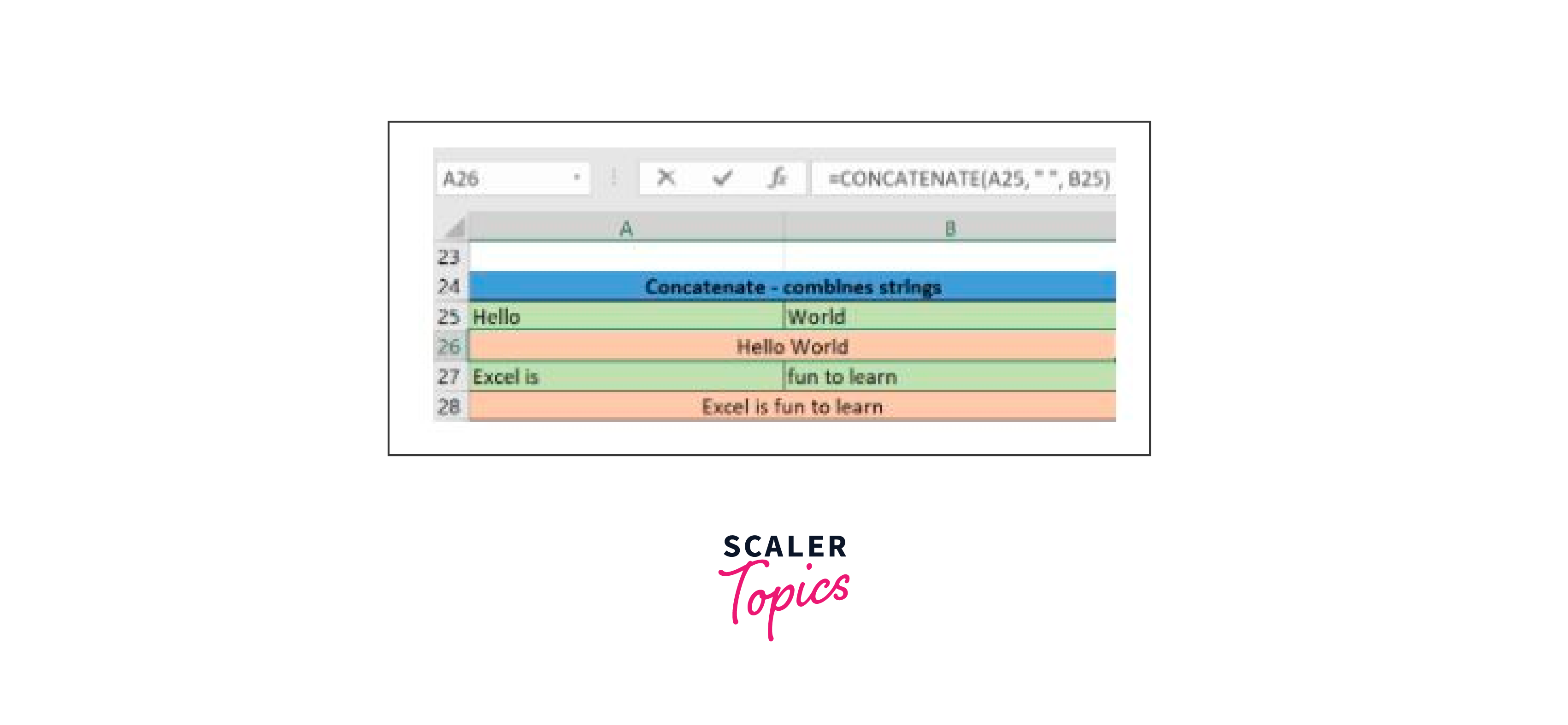
9. CONCATENATE

This technique creates one text string by joining or merging multiple text strings. The various approaches to carrying out this task are listed below.

In the following example, we used the syntax:

"=CONCATENATE(A25, " ", B25)"

In this example, we have operated with the syntax:

"=CONCATENATE(A27&" "&B27)"

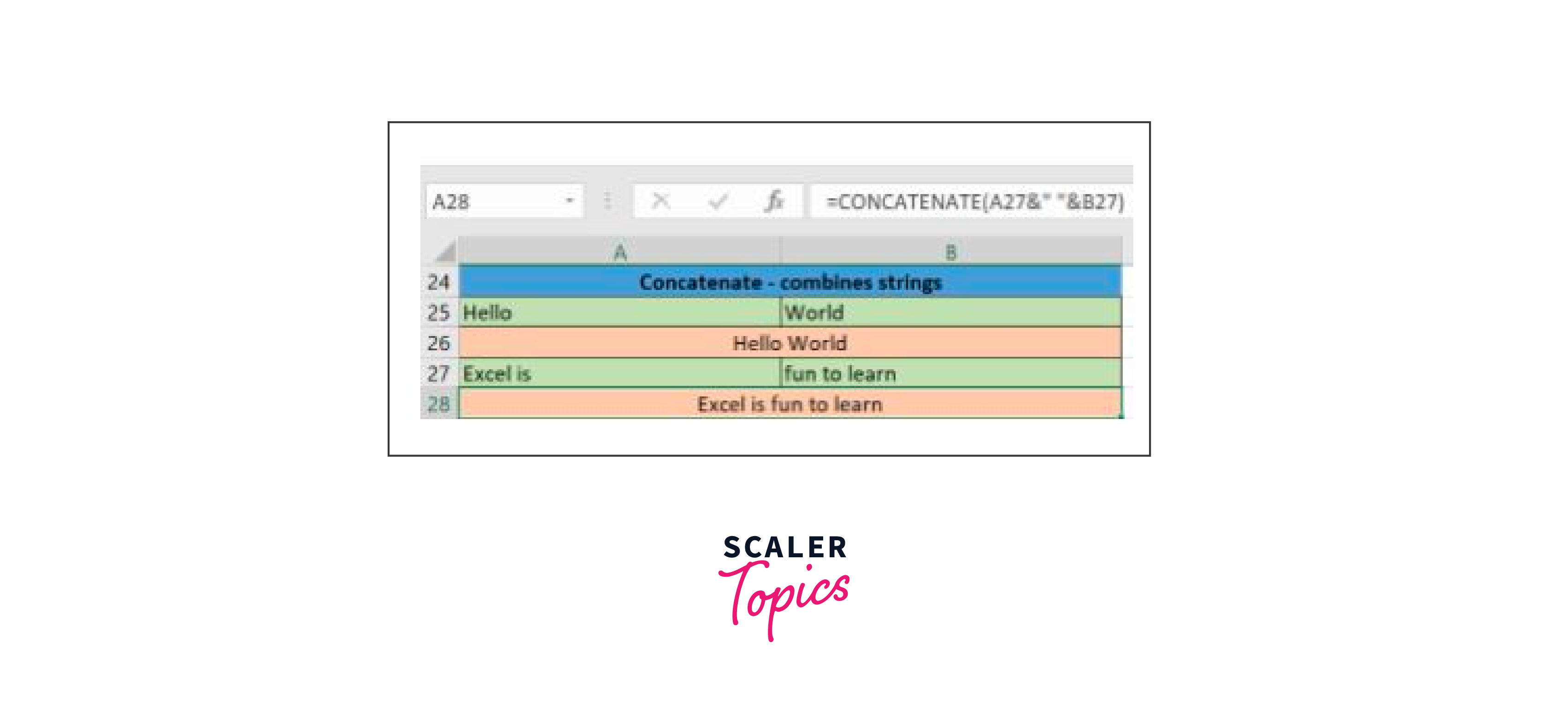
These two approaches were used to implement Excel's concatenation operation.

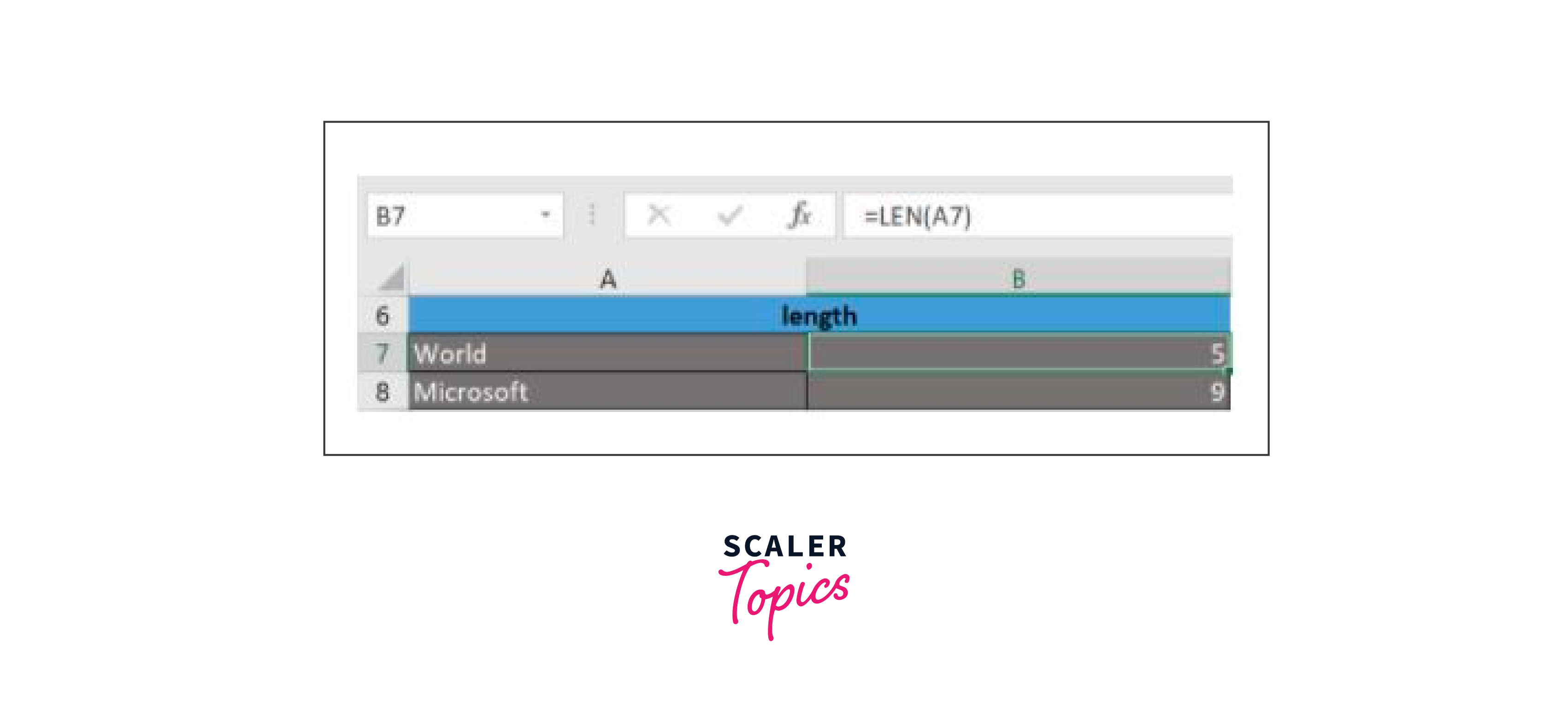
10. LEN

The function LEN() returns a string's overall character count. The number of characters, including spaces and special characters, will be counted. An example of the Len function is provided below.

Let's move on to the following Excel feature on our article's list.

11. REPLACE

The REPLACE() method does exactly what its name implies: it replaces a portion of a text string with another.

"=REPLACE(old_text, start_num, num_chars, new_text)" is the syntax.

Start_num, in this case, refers to the index position from which you wish to begin replacing the characters. Num_chars then indicate the number of characters you want to replace.

Let's examine the applications for this function.

Here, we are typing B101 in place of A101.

“=REPLACE(A15,1,1,"B")”

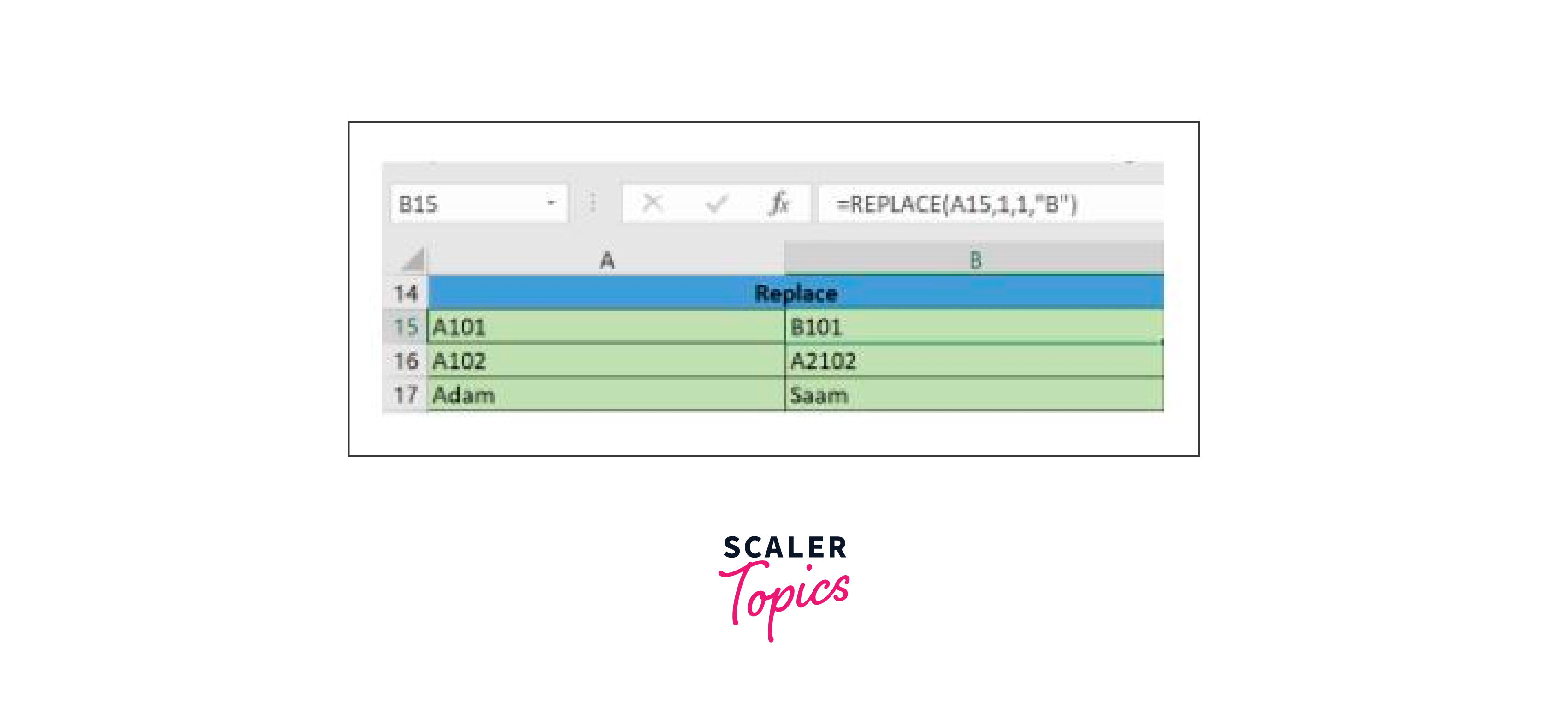
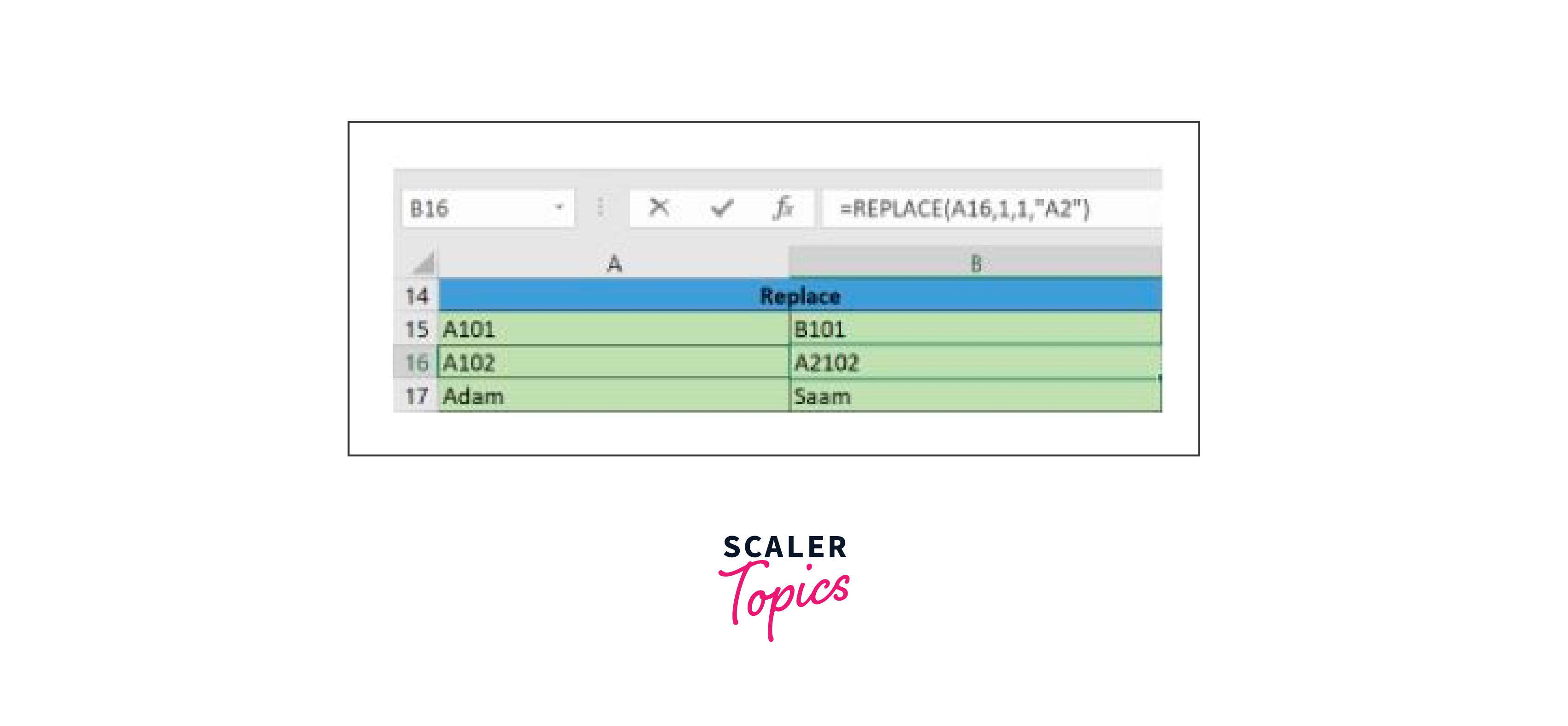
Next, by entering the following code: we are changing A102 to A2102

“=REPLACE(A16,1,1, "A2")”

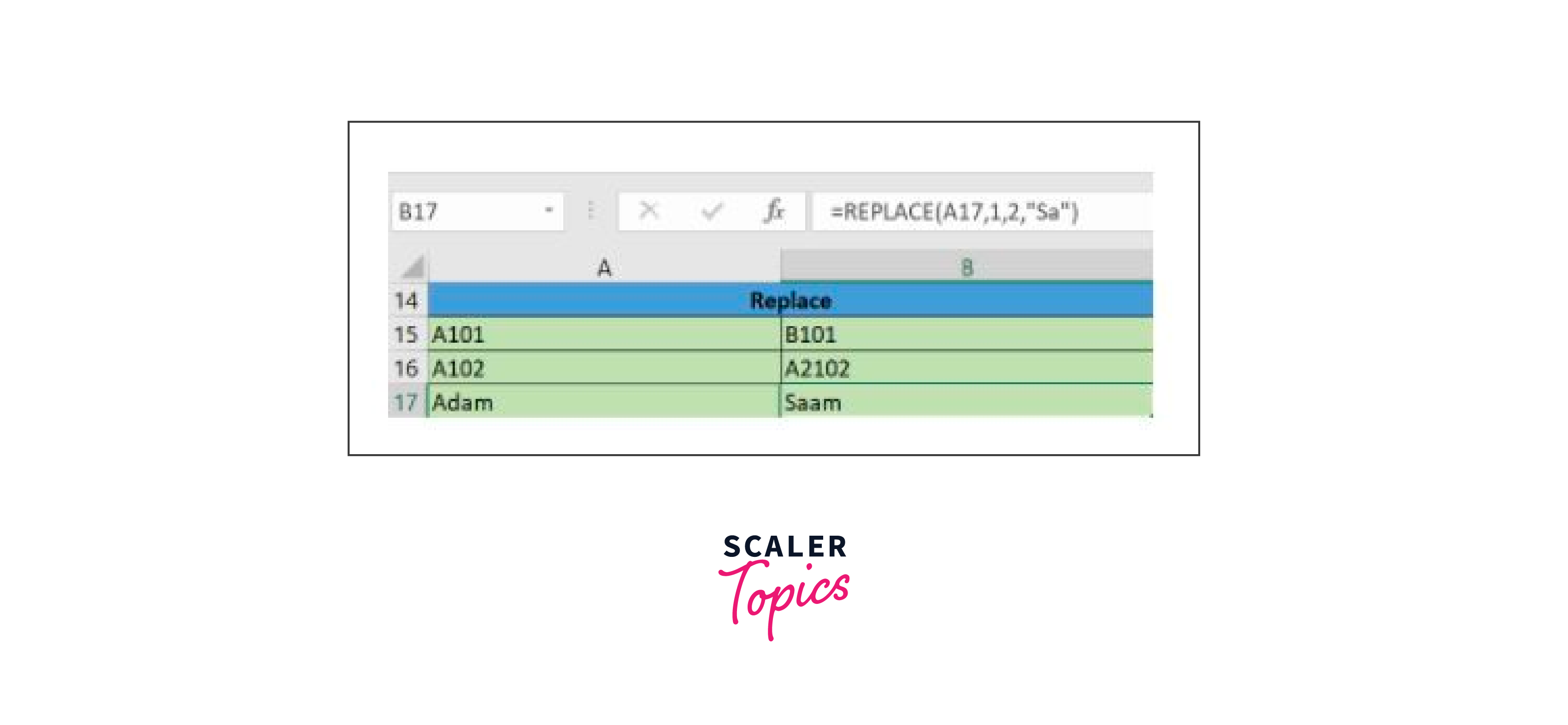
Finally, by entering: we are changing Adam to Saam.

“=REPLACE(A17,1,2, "Sa")”

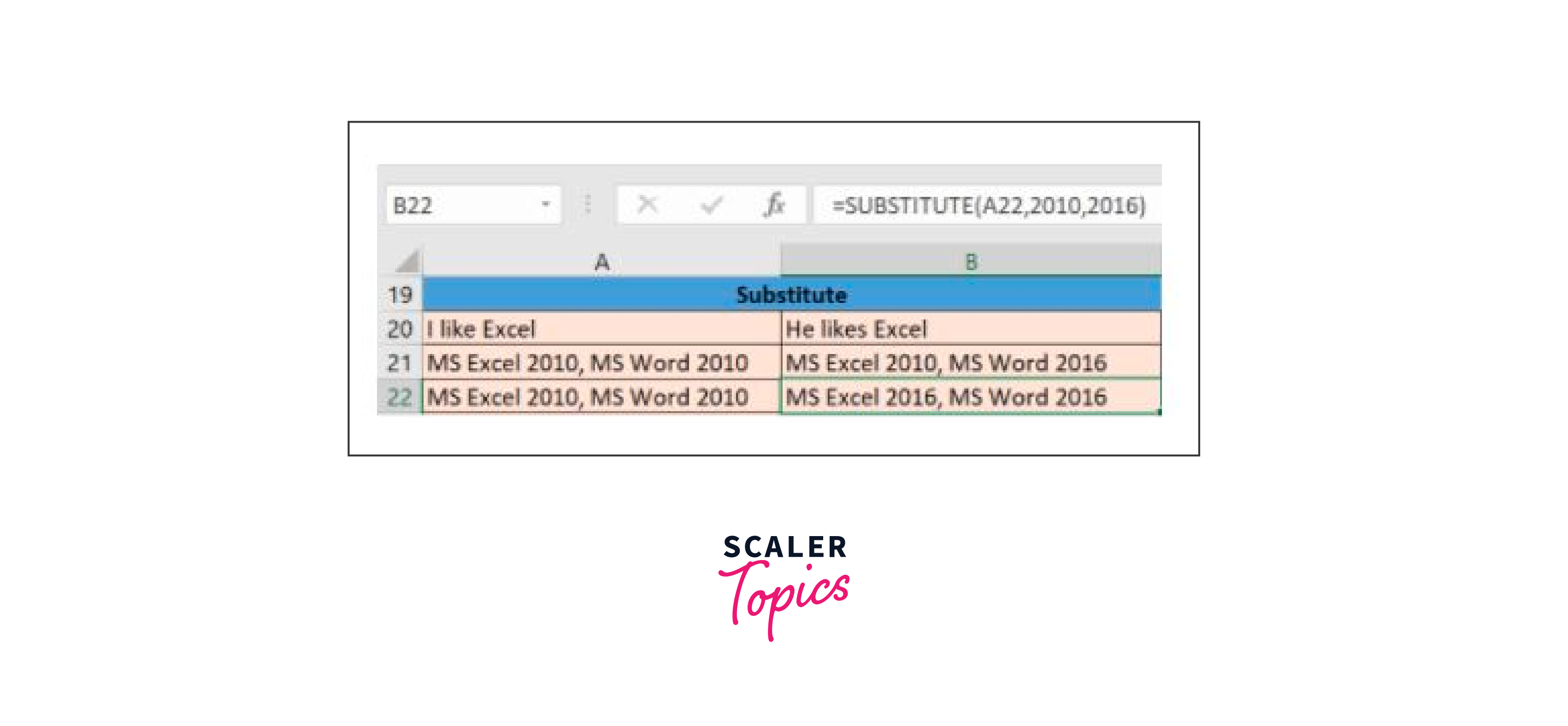
12. SUBSTITUTE

In a text string, the SUBSTITUTE() function substitutes new text for old text.

"=SUBSTITUTE(text, old_text, new_text, [instance_num])" is the syntax.

Here, [instance_num] makes several references to the index position of the current texts.

Several instances of this function are provided below:

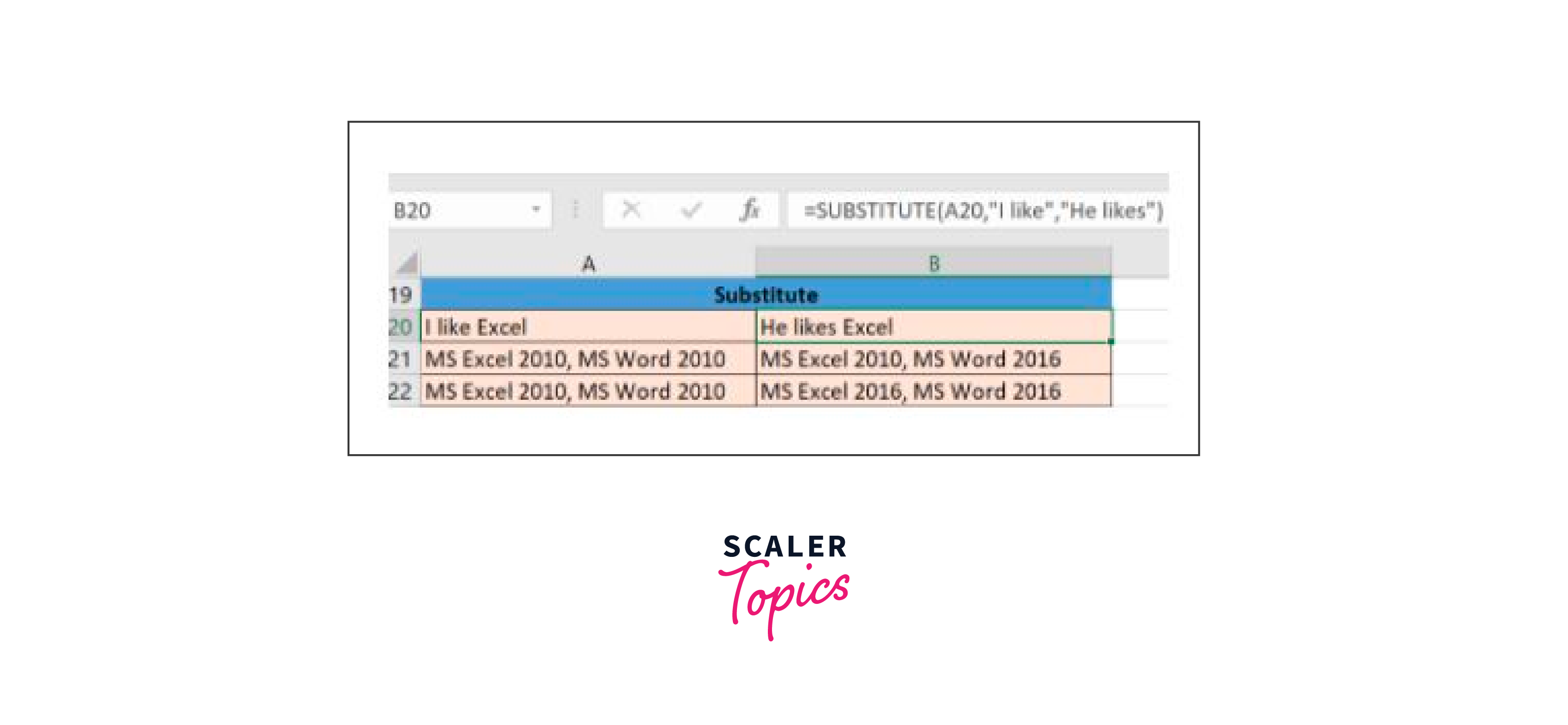
Here, we are typing: but replacing "I like" with "He likes"

“=SUBSTITUTE(A20, "I like","He likes")”

Next, we will enter "=SUBSTITUTE(A21,2010,2016,2)" to replace the second 2010 that appears in the original text in cell A21 with 2016.

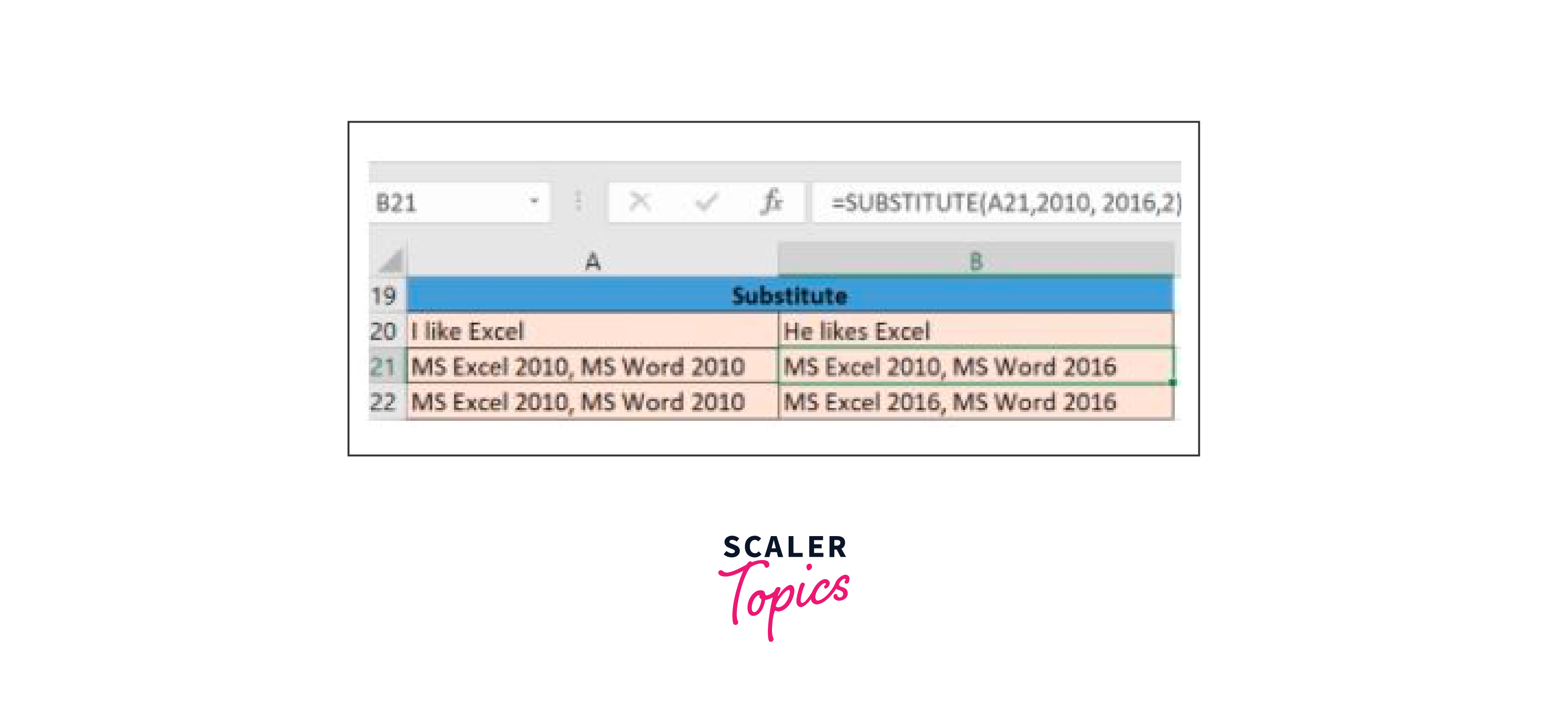
Type "=SUBSTITUTE(A22,2010,2016)" to replace the 2010s in the original text with 2016.

Now that we have covered the substitute function in detail let's move on to our next function.

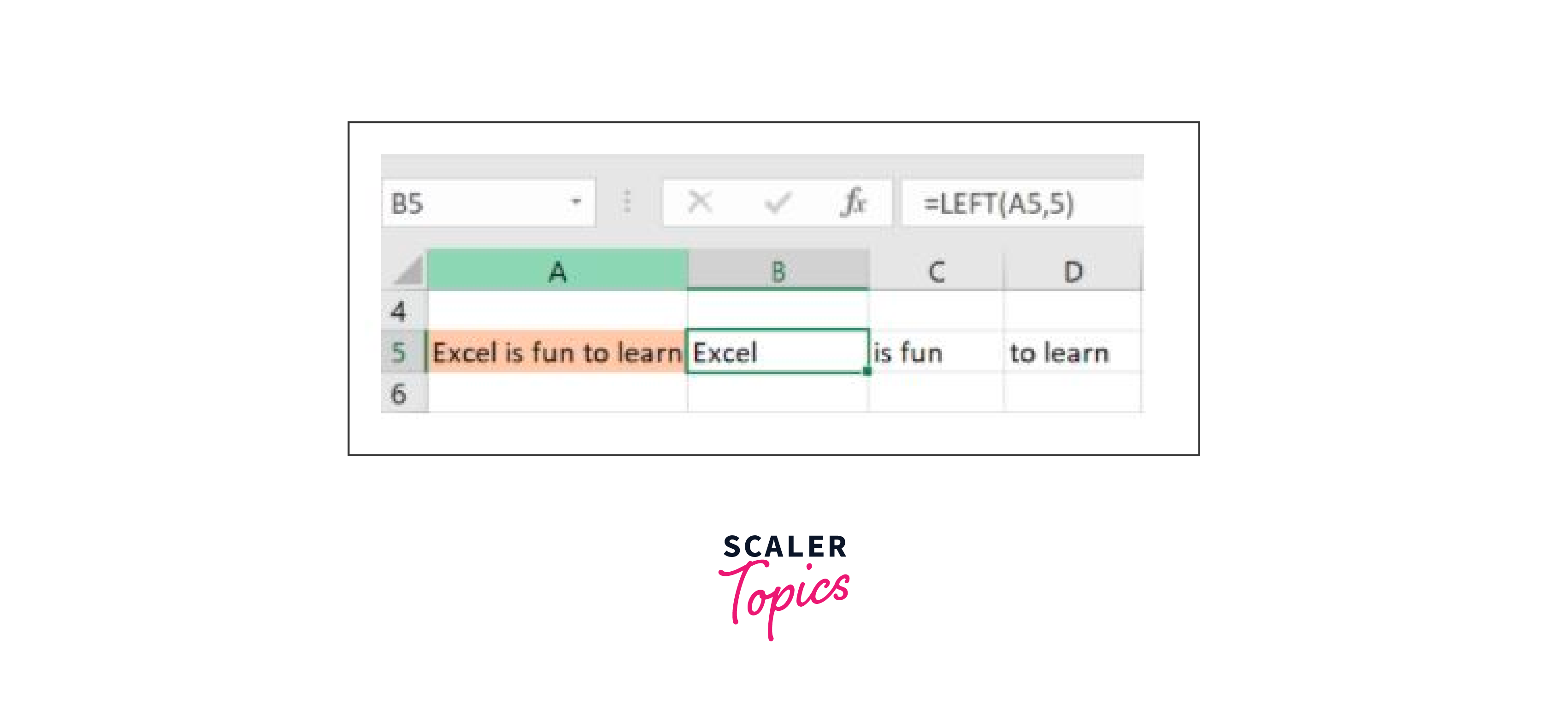
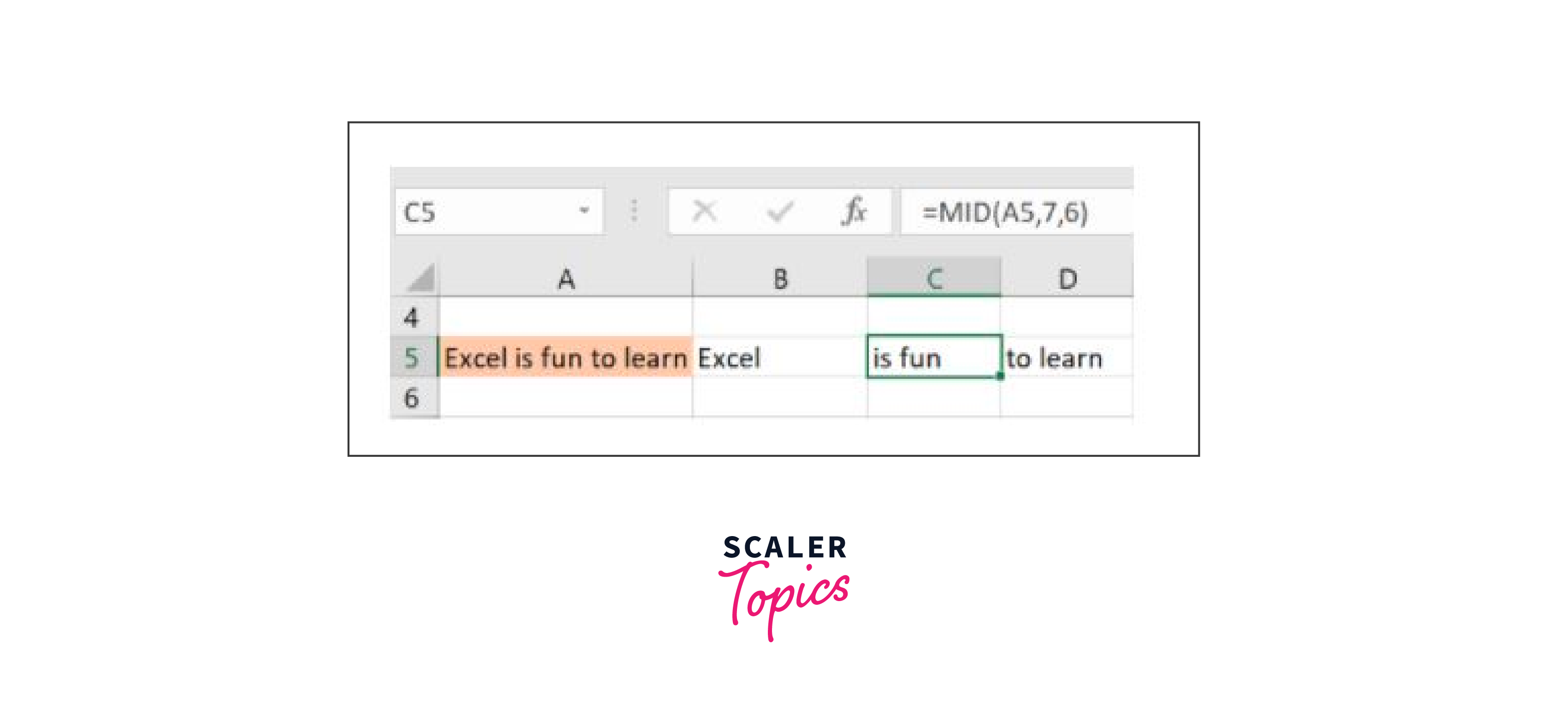
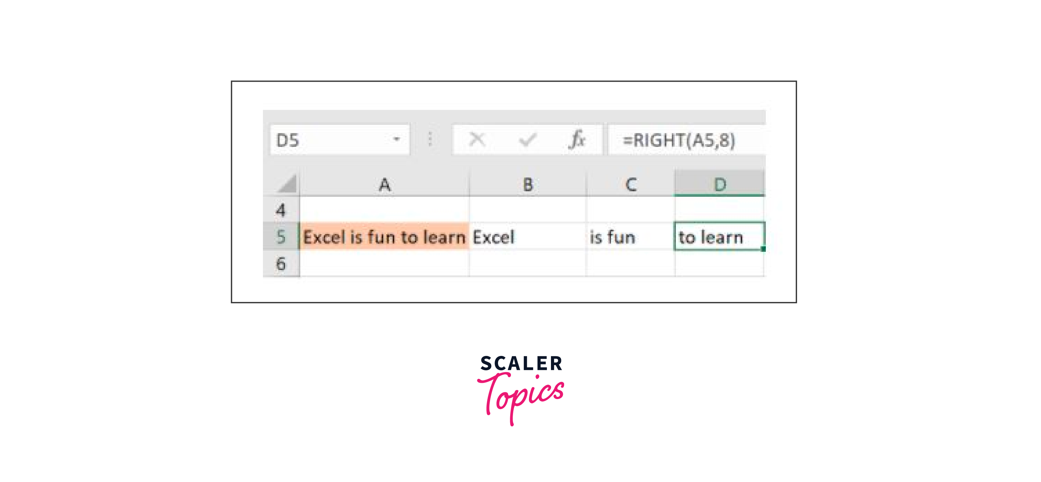
13. LEFT, RIGHT, MID

The LEFT() function provides the text string's starting character count. In contrast, the MID() method, given a beginning location and length, returns the characters from the middle of a text string. The right() function also returns how many characters are left in a text string.

Let's use a few examples to understand these functions better.

The example below uses the left function to get the sentence's leftmost word in cell A5.

An example of how to use the mid function is provided below.

Here is an example of the appropriate function.

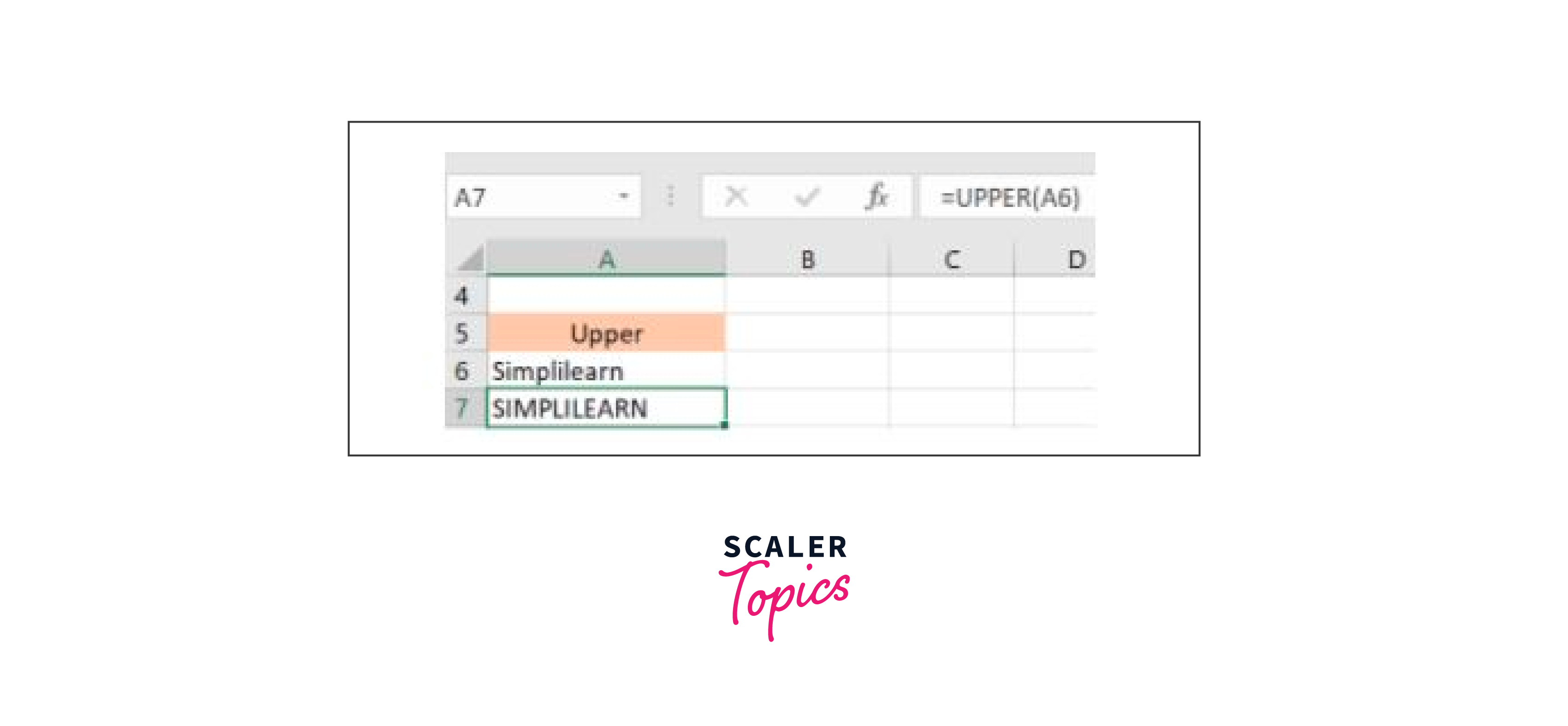
14. UPPER, LOWER, PROPER

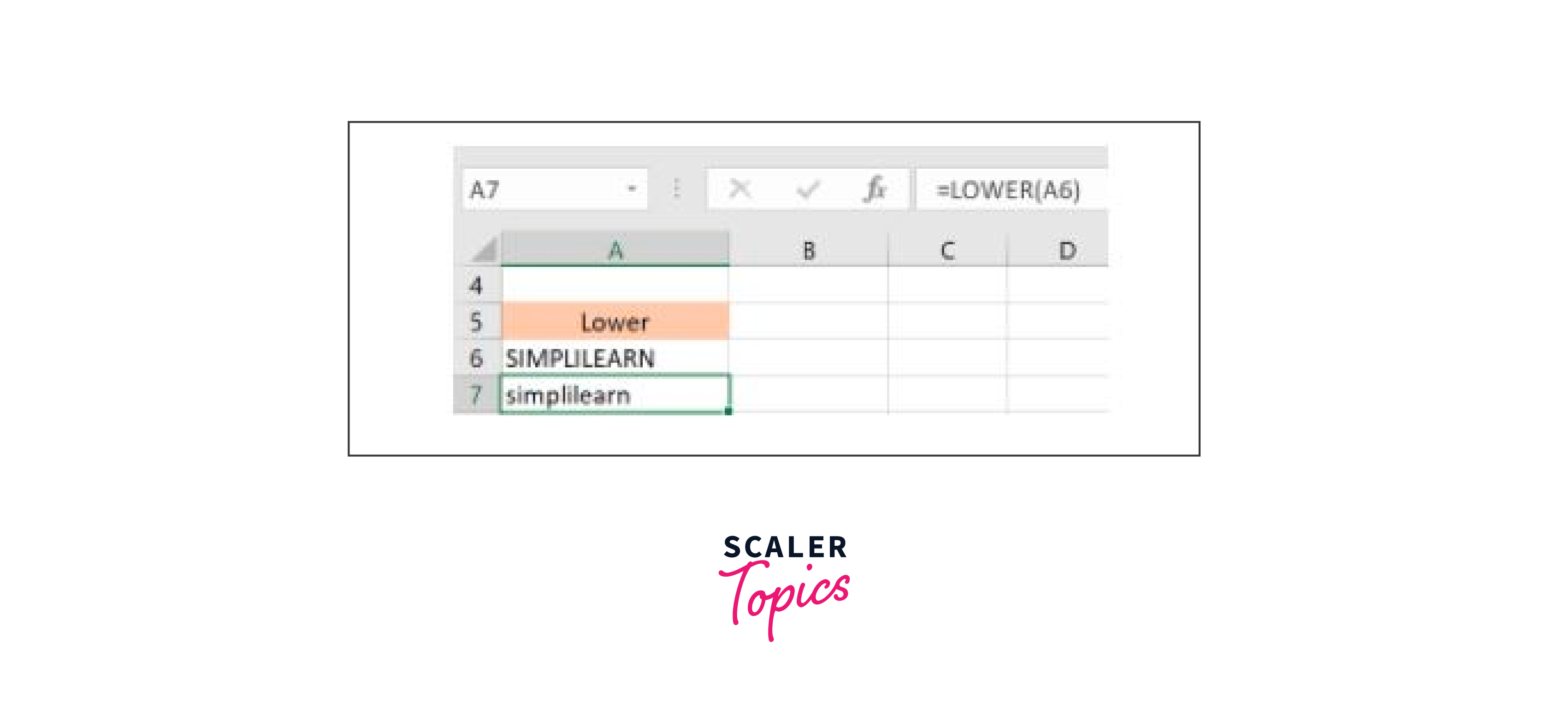
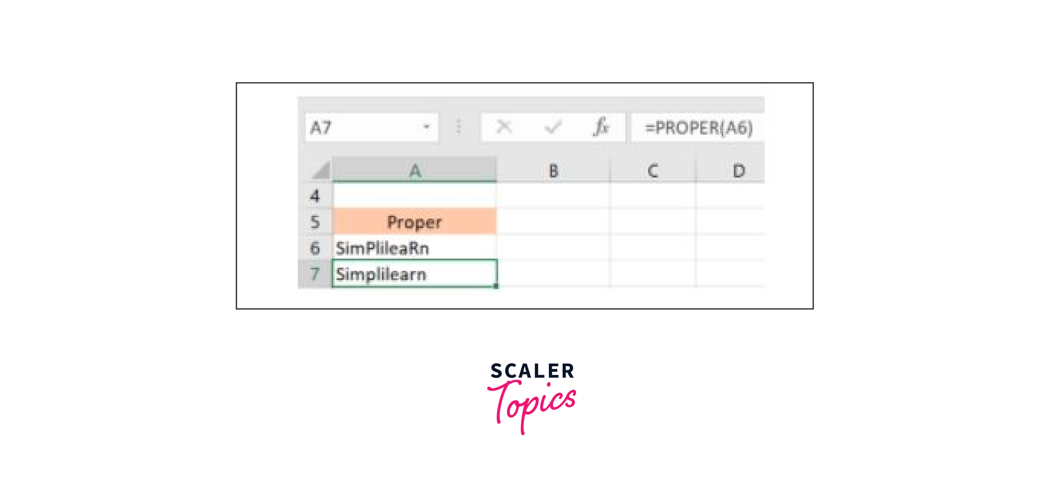
Any text string can be made uppercase using the UPPER() function. The LOWER() function, in contrast, lowercase any text string. Any text string can be converted to the proper case using the PROPER() function; this means that the first letter of each word will be in uppercase, and all other letters will be in lowercase.

Let's use the following examples to comprehend this better:

Here, the text in A6 has been changed to text in all uppercase in A7.

As shown in A7, we have changed the text in A6 to all lowercase.

Last, we changed the incorrect text in A6 to a clean and appropriate structure in A7.

Let's explore some date and time operations in Excel right away.

15. NOW()

Excel's NOW() function provides the current system date and time.

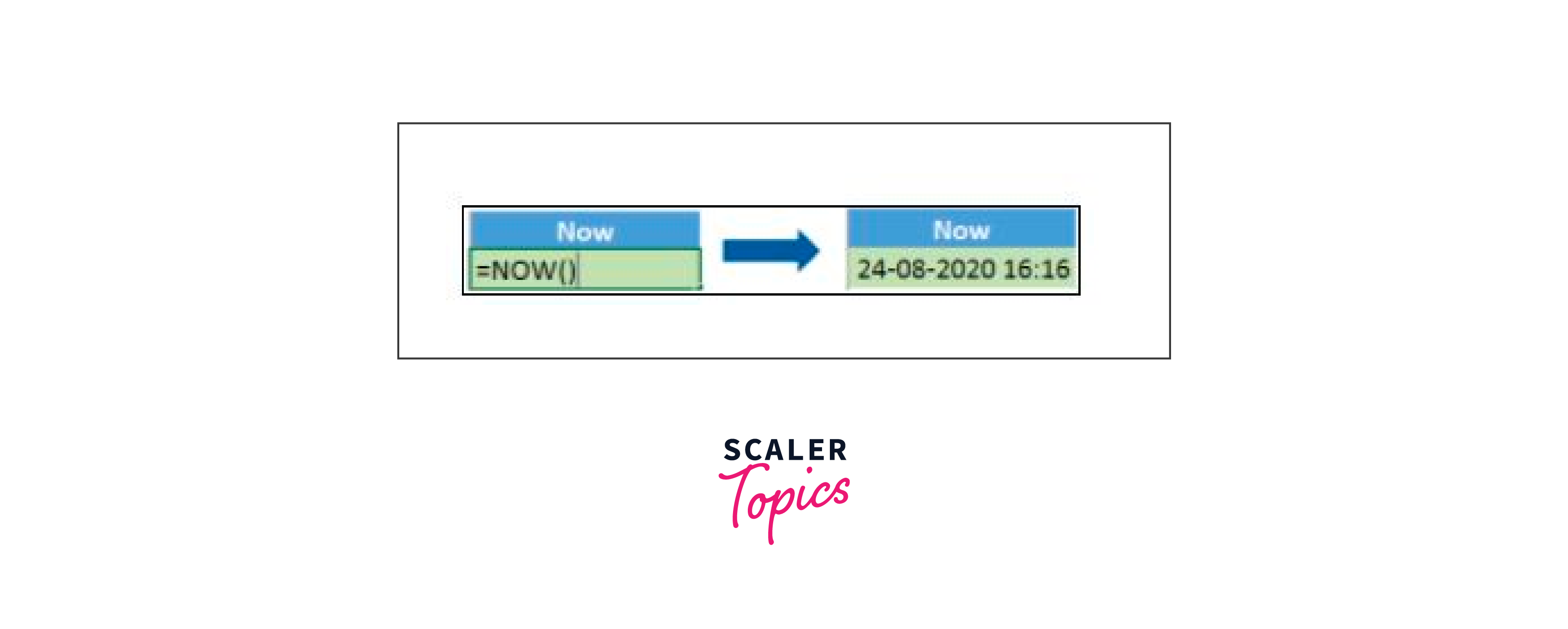
Your system's date and time will affect the NOW() function's output.

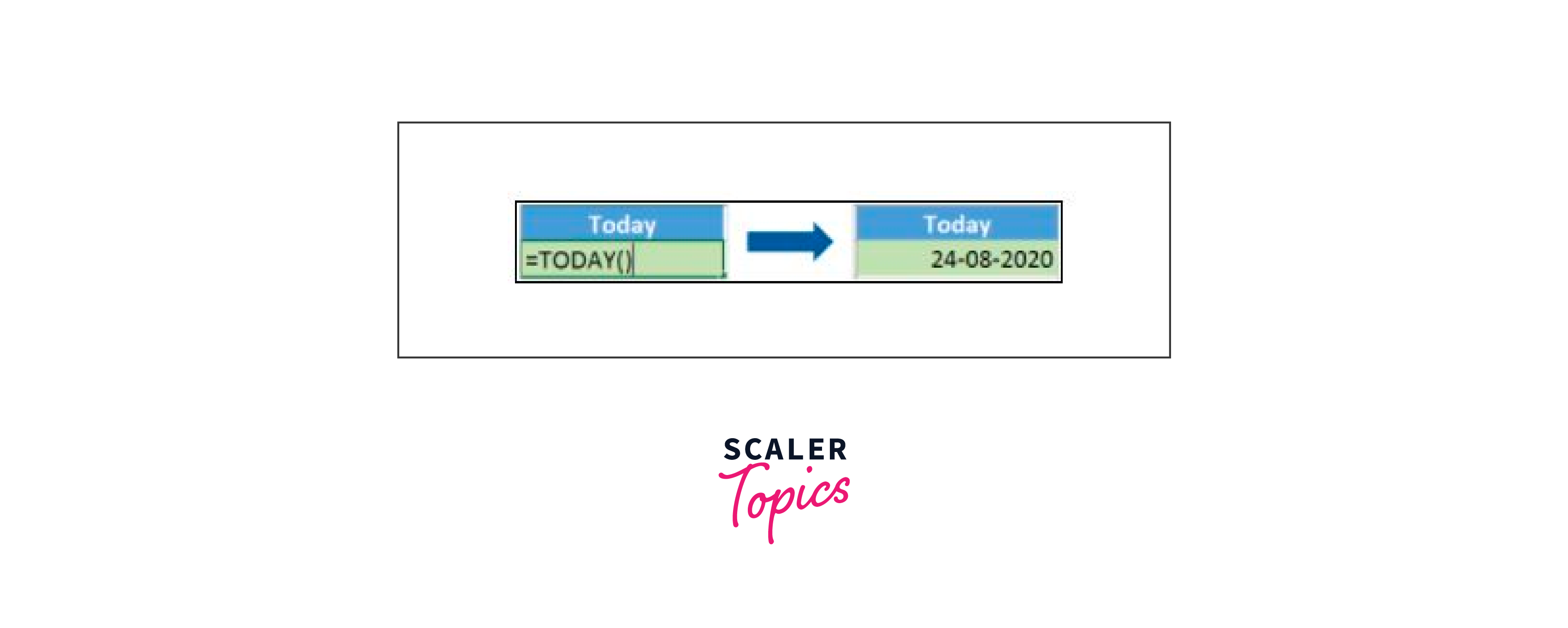
16. TODAY()

The current system date is provided via Excel's TODAY() function.

The objective The day of the month is returned by the function DAY(). The value will fall between 1 and 31. The first day of the month is 1, and the last day is 31.

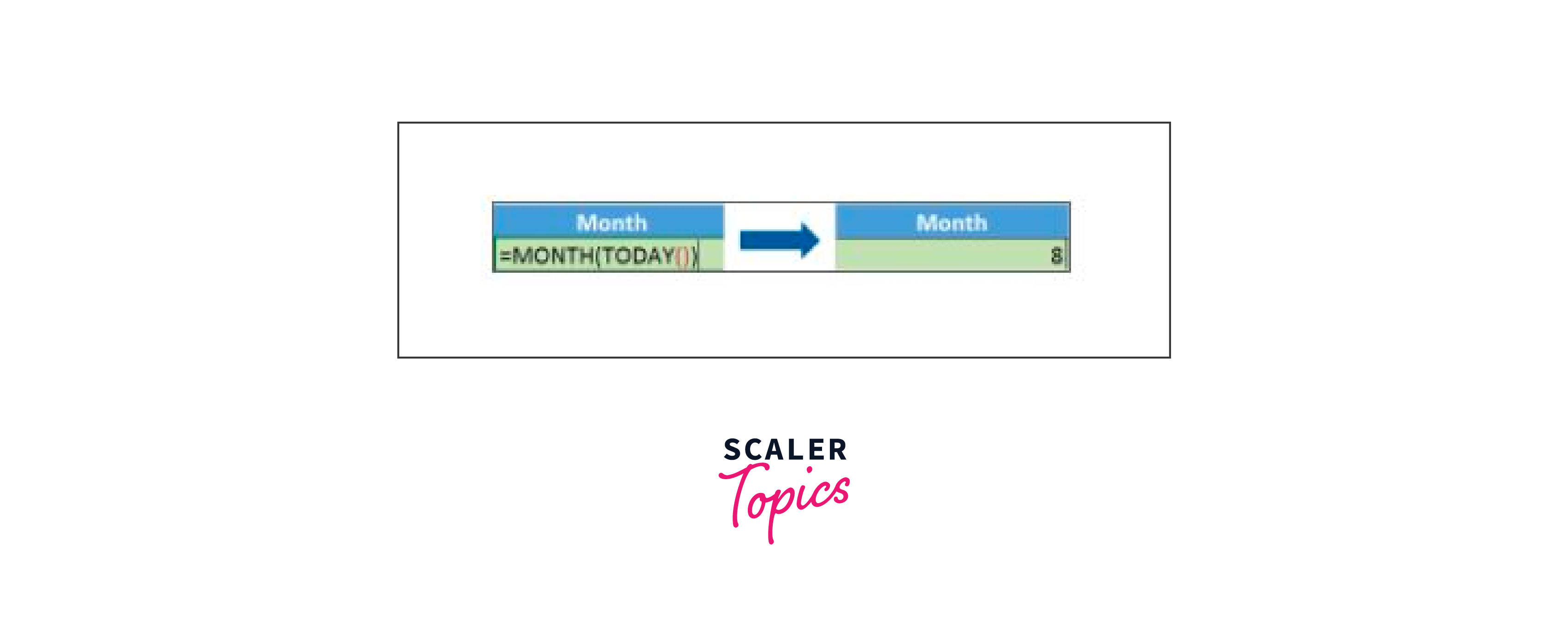
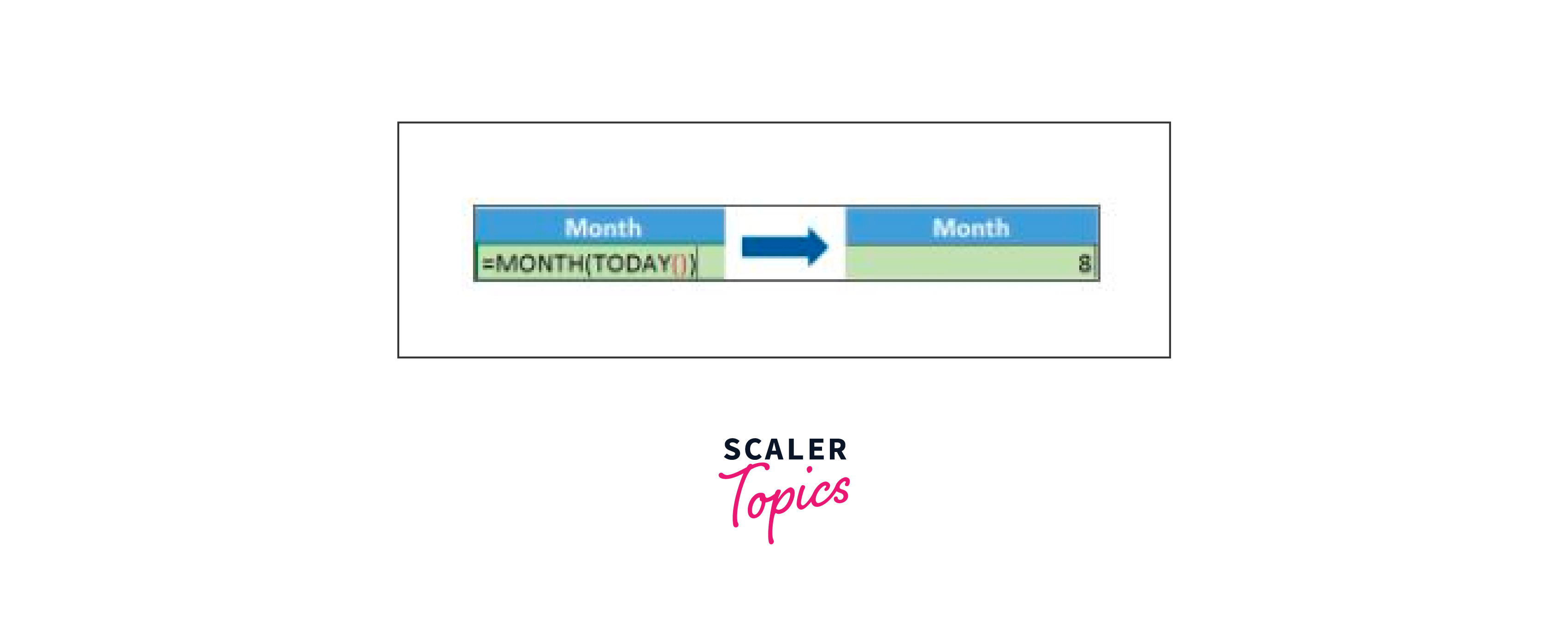
The month is returned by the MONTH() method as a number between 1 and 12, with 1 denoting January and 12 denoting December.

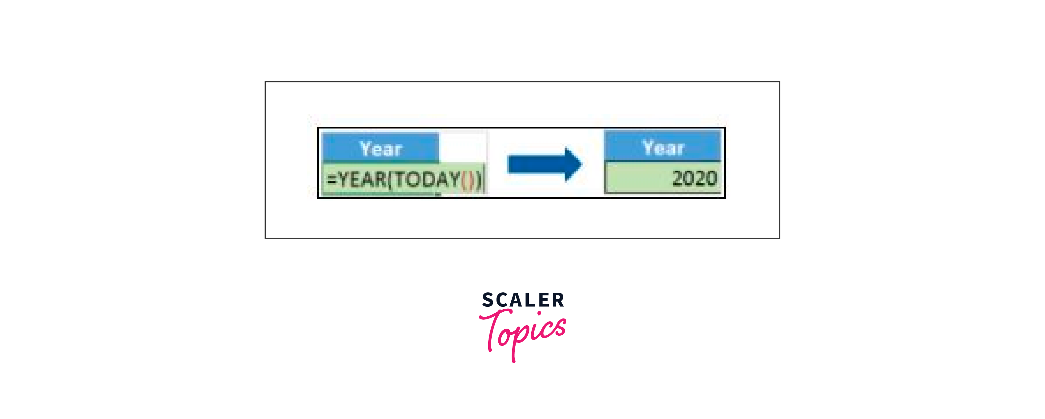
As its name implies, the YEAR() function gets the year from a date value.

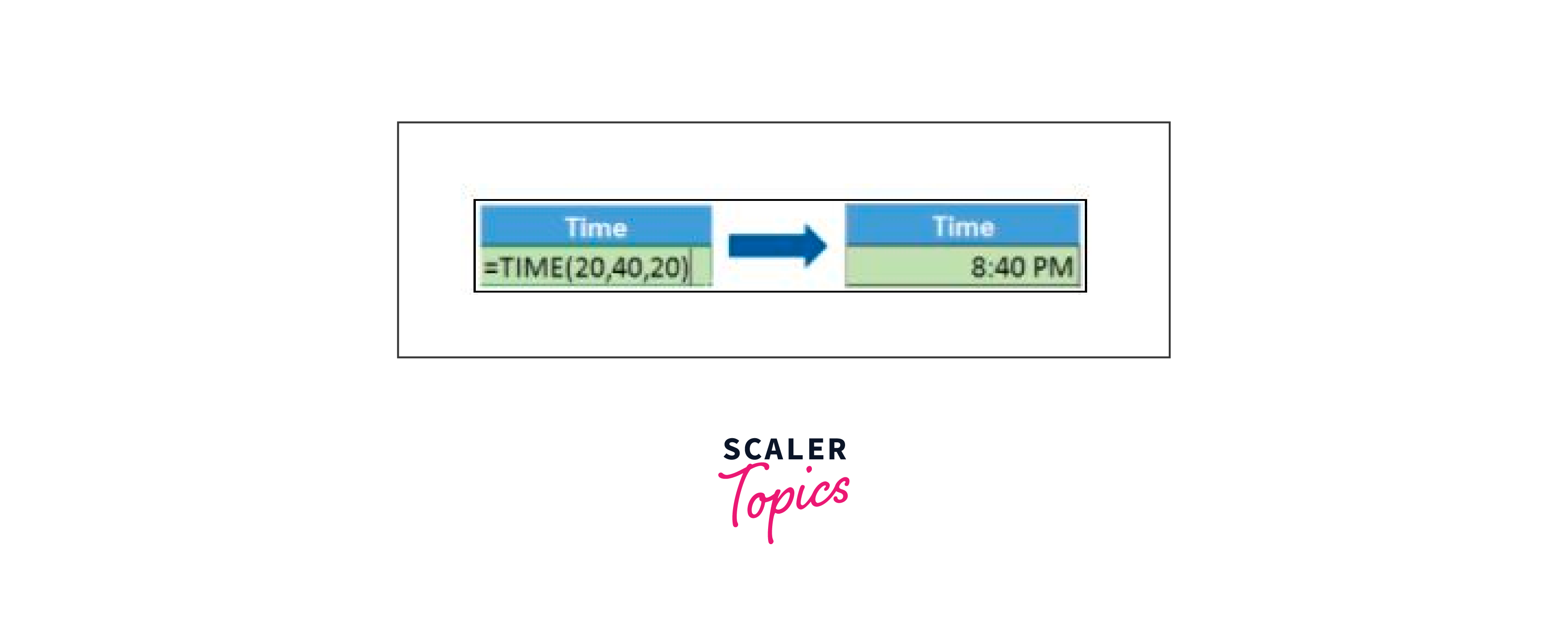
17. TIME()

Hours, minutes, and seconds are converted into an Excel serial number with a time format using the TIME() function.

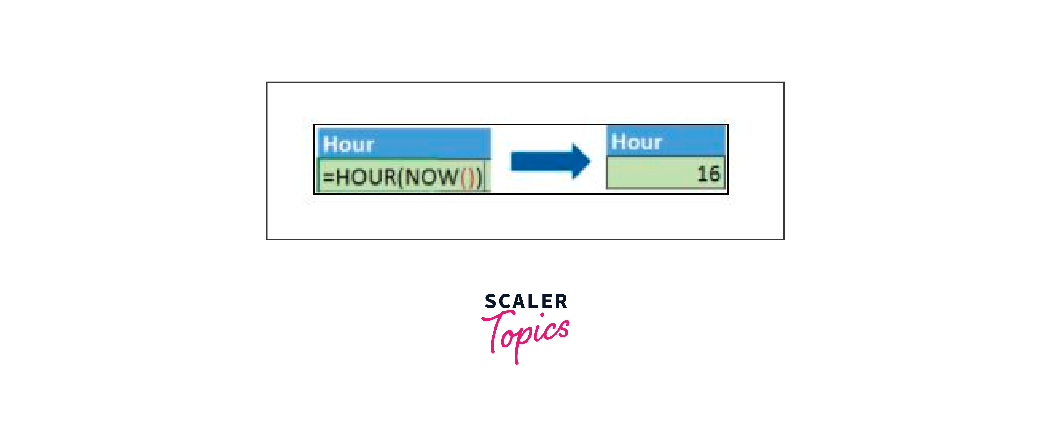
18. HOUR, MINUTE, SECOND

The HOUR() function produces the hour from a time value as a number between 0 and 23. Here, 0 denotes 12 AM, while 23 denotes 11 PM.

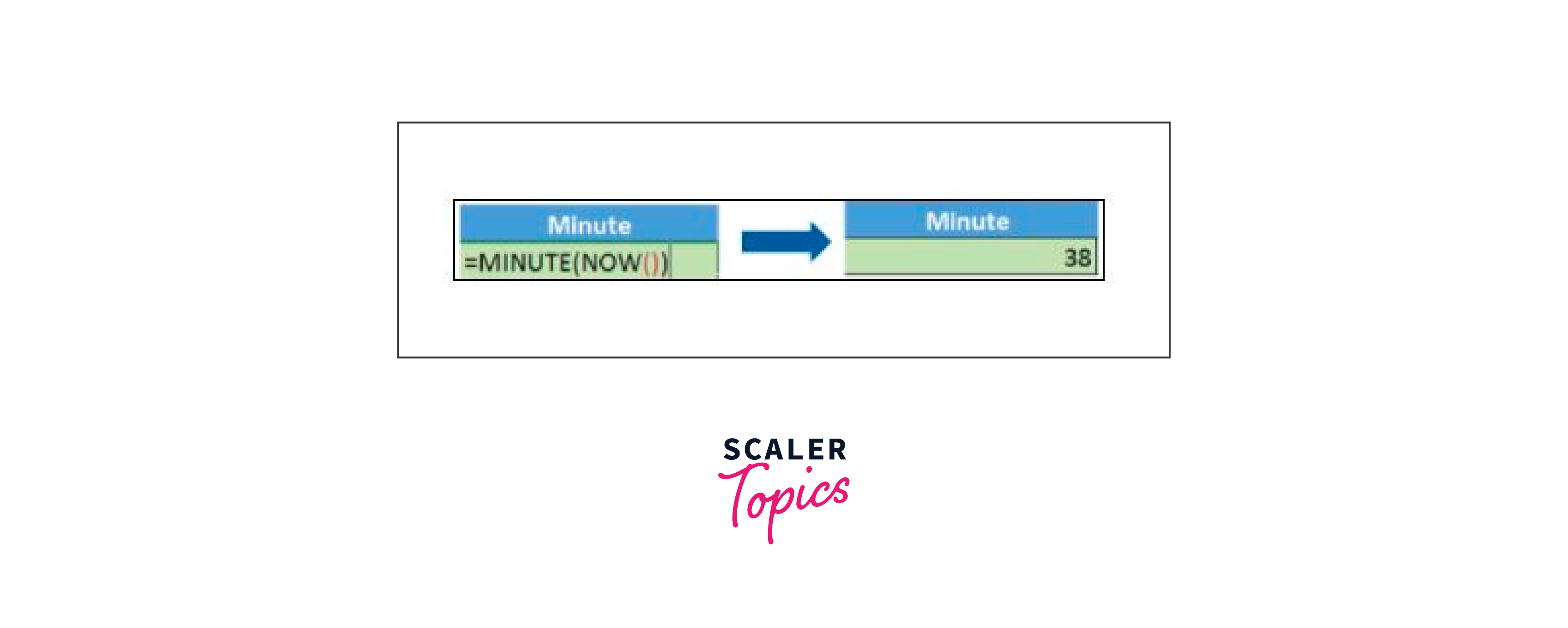
The MINUTE() function extracts the minute from a time value and returns it as an integer between 0 and 59.

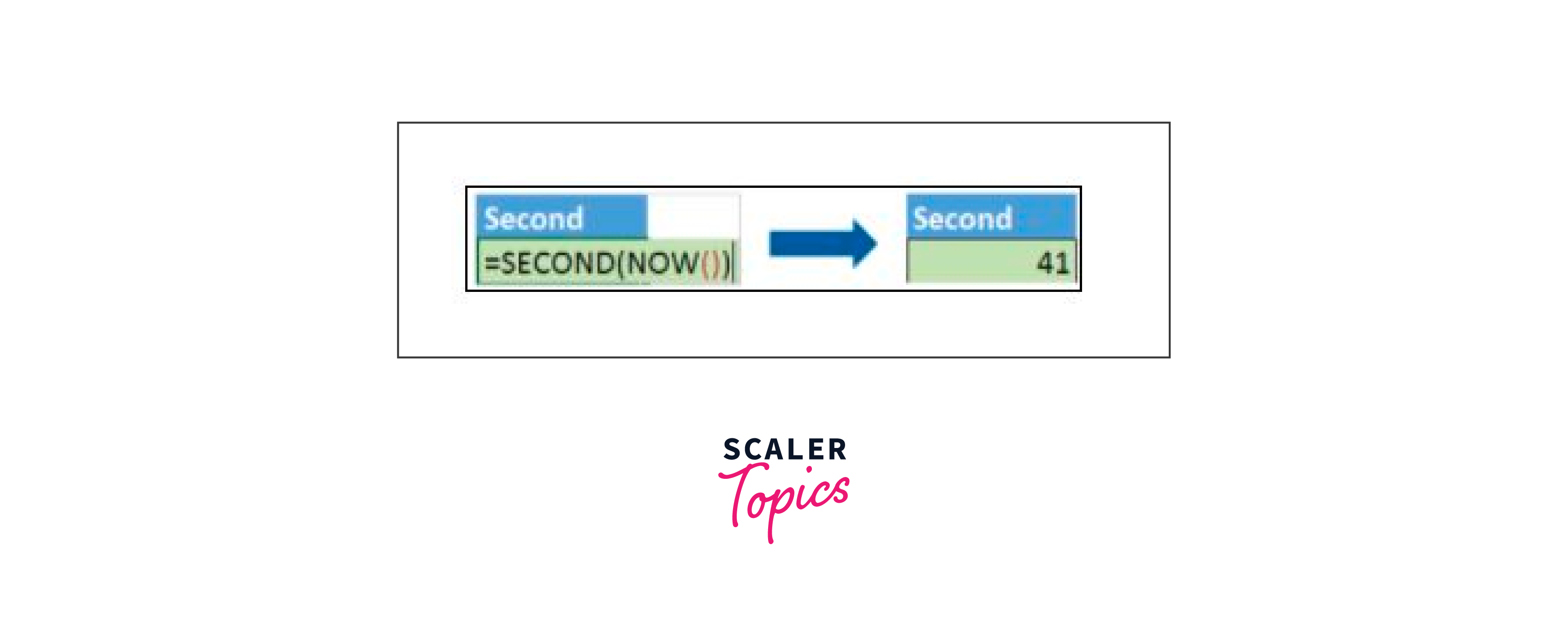
The second from a time value is returned by the SECOND() function as an integer between 0 and 59.

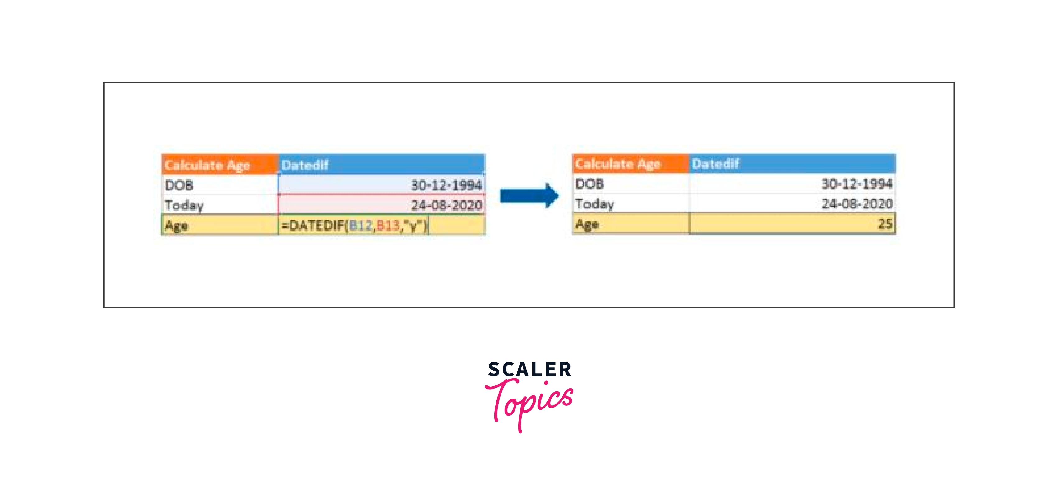
19. DATEDIF

The DATEDIF() method calculates the difference in years, months, or days between two dates.

Here is an example of a DATEDIF function that determines a person's current age based on their birthdate and the current date.

Review a few crucial advanced Excel functions frequently used to analyze data and produce reports.

20. VLOOKUP

The VLOOKUP() function is covered in this article after that. This is an acronym for the vertical lookup, which searches the leftmost column in a table for a specific value. It then returns a value from the specified column in the same row.

The arguments for the VLOOKUP function are listed below:

• lookup_value: This is the value that has to be found in a table's first column.
• table - The table from which the value is fetched is indicated by this.
• col_index - The table column from which the value should be obtained.
• [Optional] range_lookup TRUE indicates a close match (the default). Exact match = FALSE.

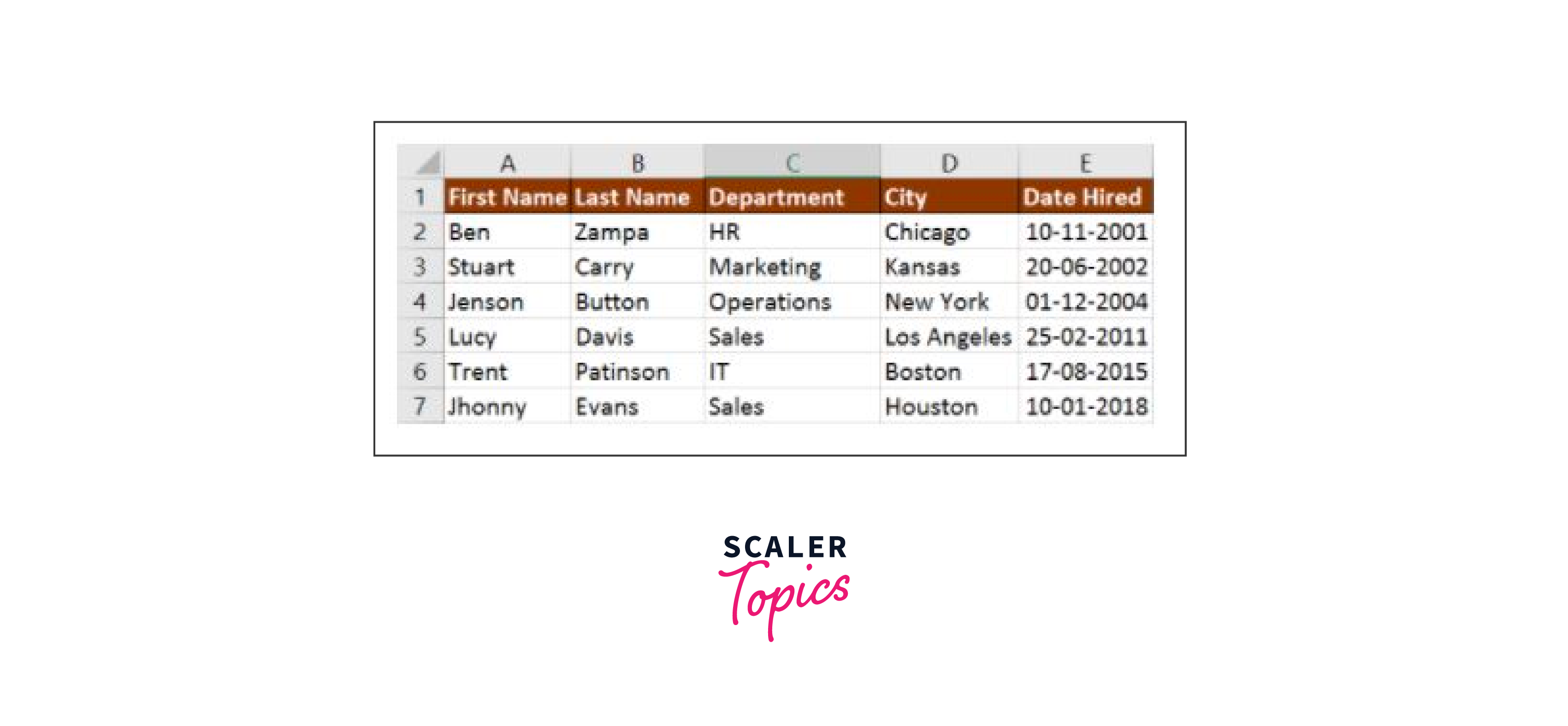
The table below will be used to demonstrate how the VLOOKUP function functions.

You might use the VLOOKUP function as displayed below to determine the department to which Stuart belongs:

Here, the lookup value is in cell A11, the table array is in cell A2, the department information is in column index number 3, and the range lookup is in cell 0 of the table.

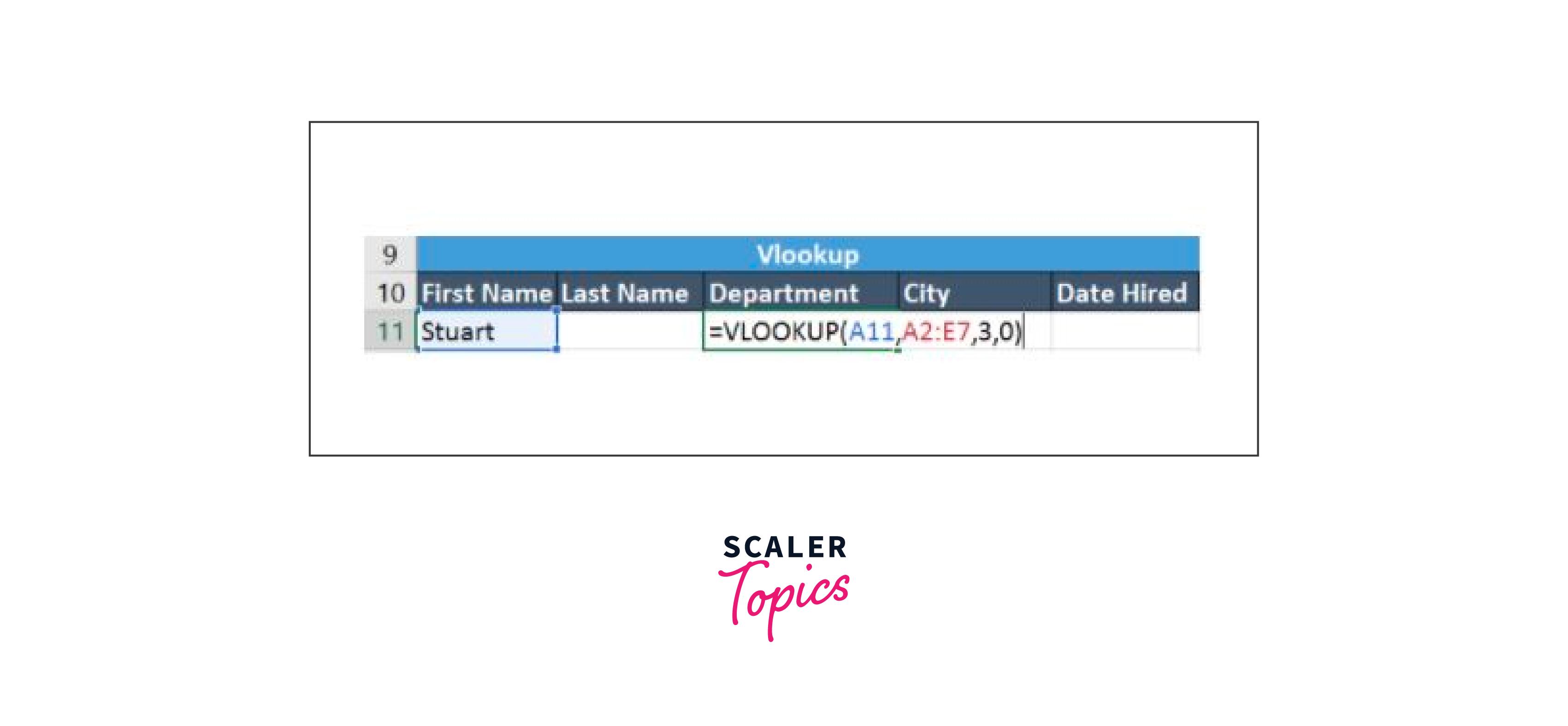
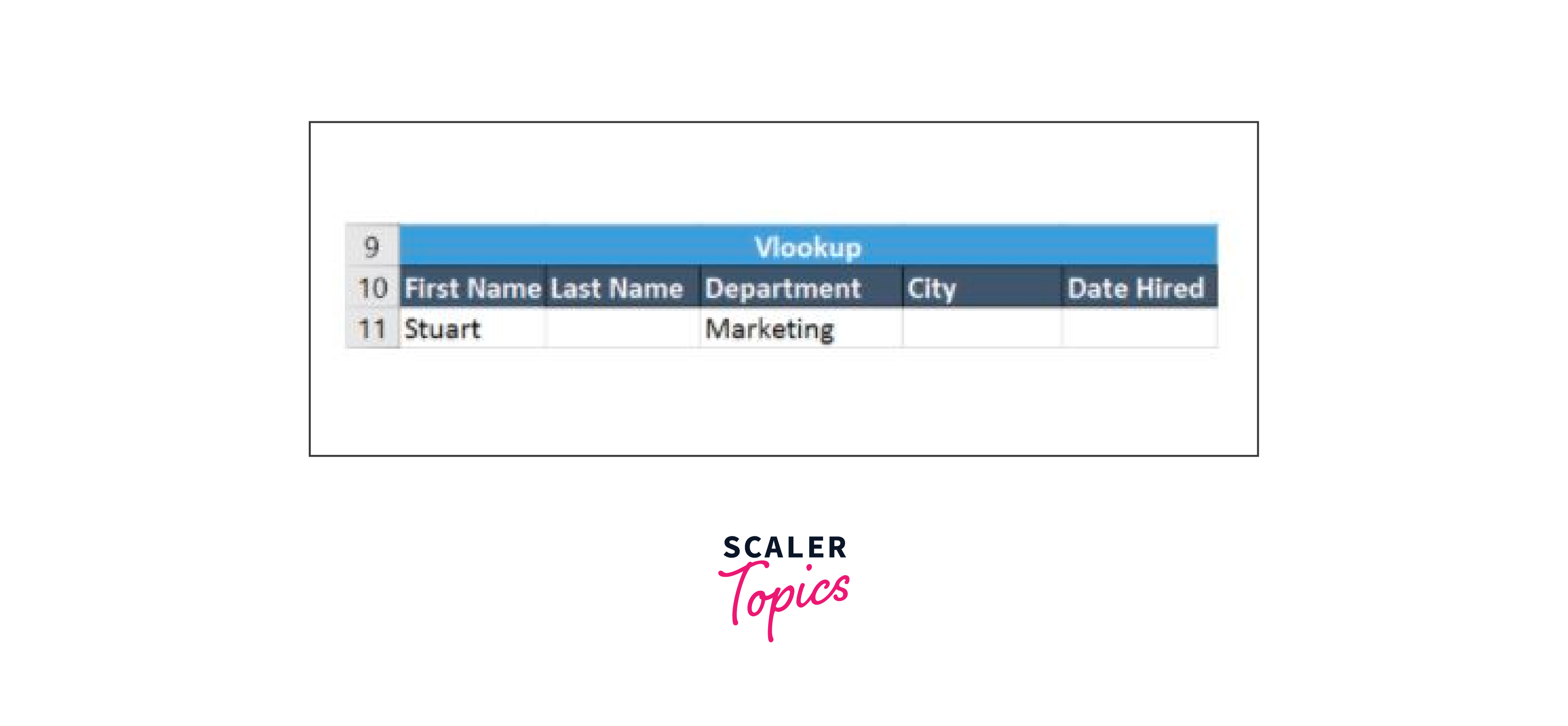
If you press enter, "Marketing" will appear, suggesting that Stuart is a member of the marketing division.

21. HLOOKUP

We also have a function called HLOOKUP(), or horizontal lookup, similar to VLOOKUP. The top row of a table or array of benefits is where the HLOOKUP function looks for a value. It displays the value from the specified row in the same column.

The HLOOKUP function's arguments are listed below:

• lookup_value - The lookup value is indicated by this. The table from which you must retrieve data is called a table.
• row_index is the row number that should be used to get data.
• [Optional] range_lookup This boolean value represents an exact or approximate match. The default setting, TRUE, denotes a close match.

Given the table below, let's look at how to use HLOOKUP to locate the city of Jenson.

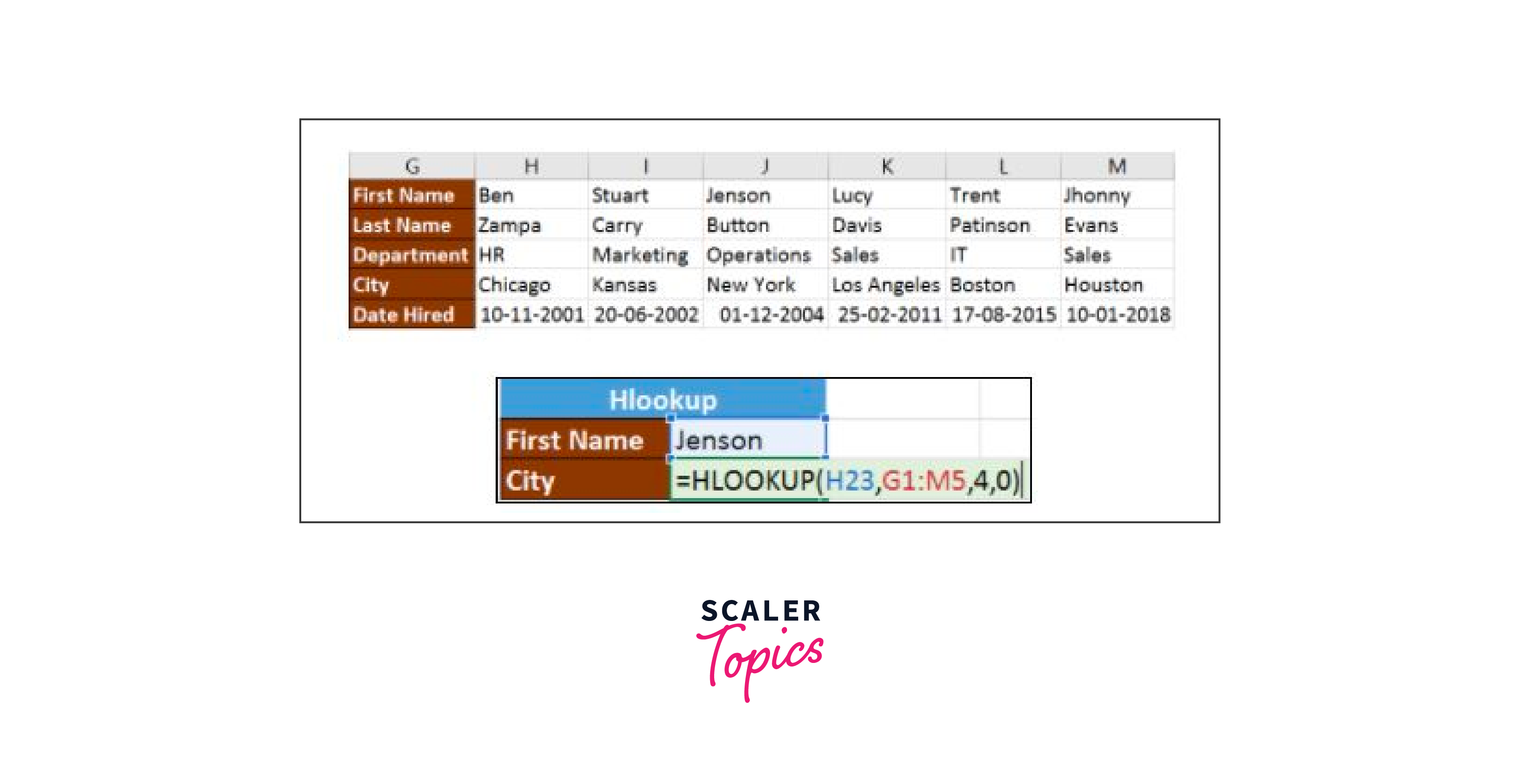
Here, H23 contains the lookup value, which is Jenson. G1 is the table array, and 4 is the row index number.

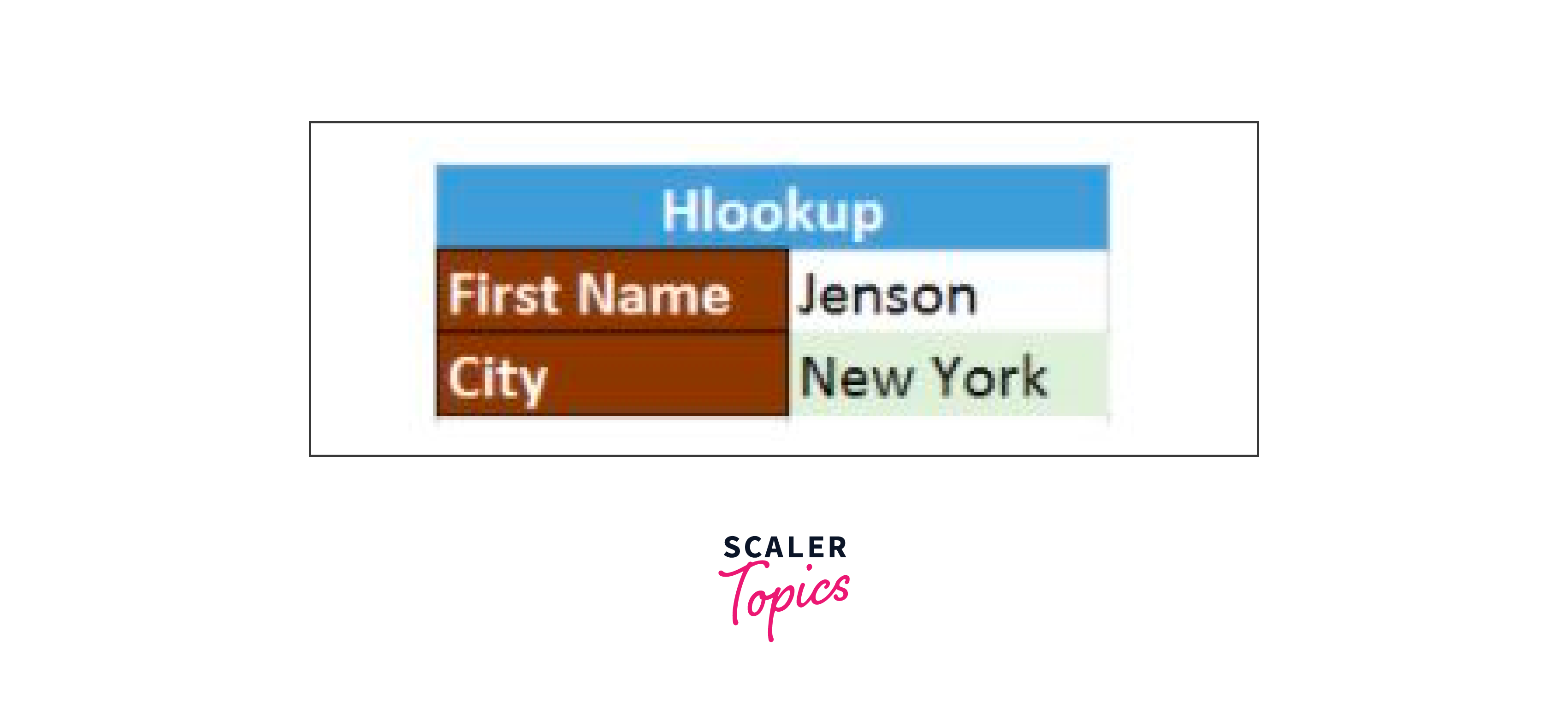
"New York" will be shown once you press enter.

22. IF Formula

If a condition is met, the IF() function verifies it and returns a specific value. If the condition is FALSE, it will return a different value.

In the example below, we wish to determine whether cell A2's value exceeds 5. The function will return "Yes 4 is greater" if greater than 5, and "No" otherwise.

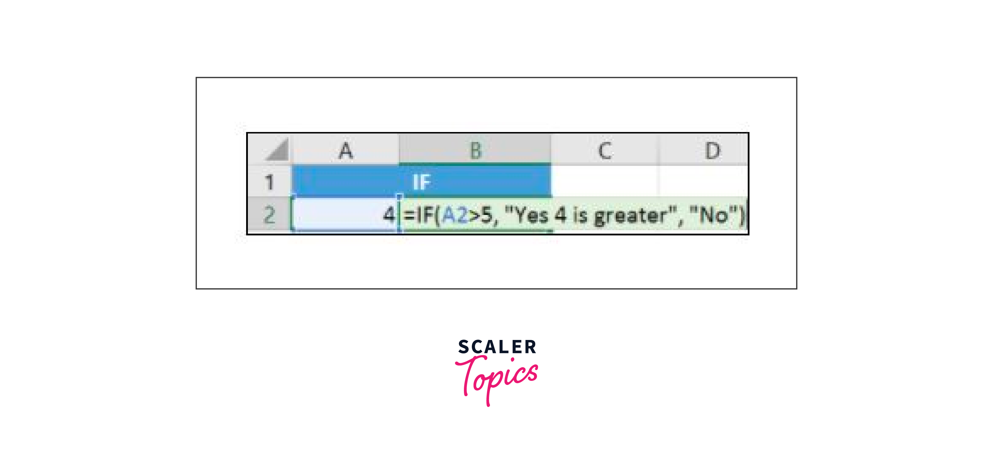
Since 4 is not larger than 5, it will, in this instance, reply "No."

Another often-used function is 'IFERROR'. If an expression evaluates to an error, this function returns a value; otherwise, it returns the expression's value.

Let's say you want to multiply 10 by 0. This formula must be corrected since a number cannot be divided by zero. It will lead to a mistake.

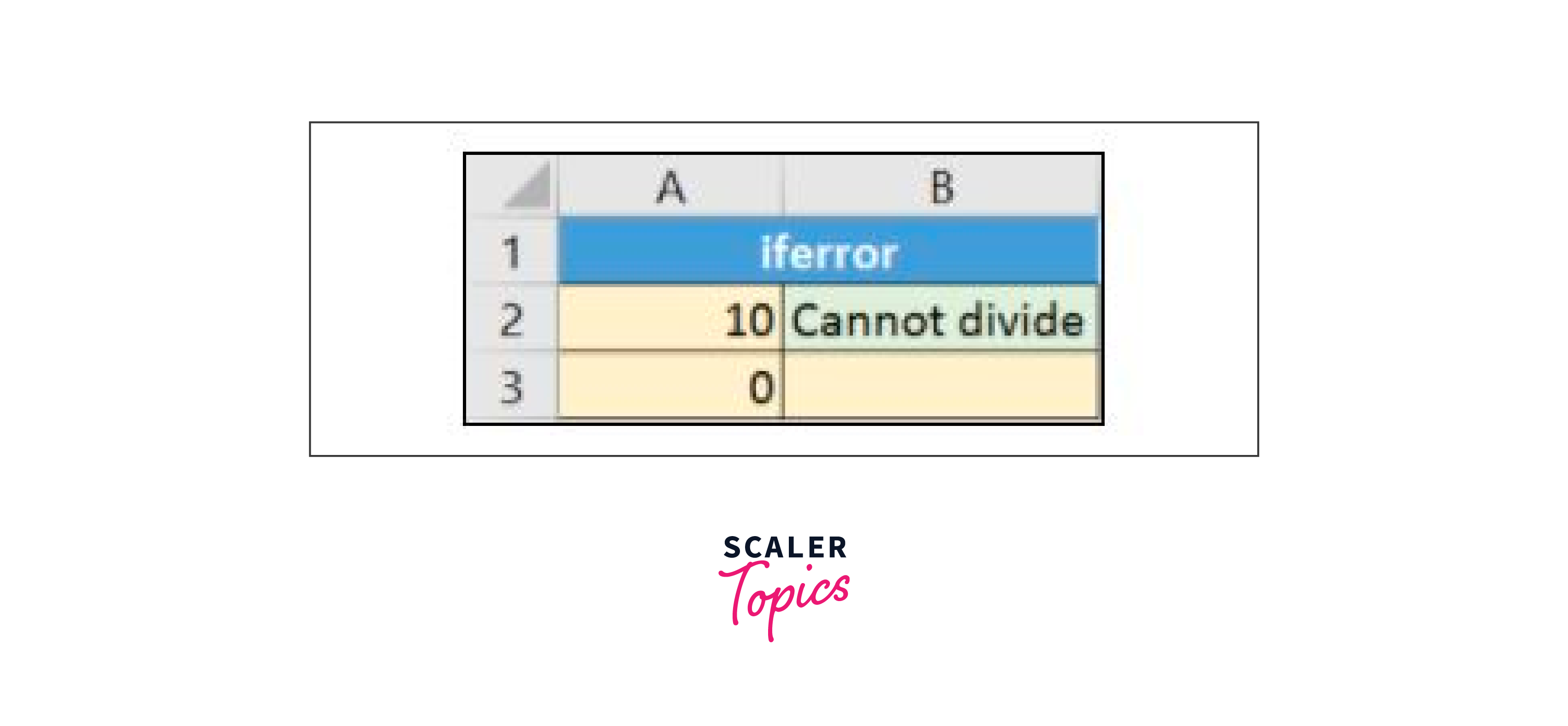
"Cannot divide" is the result of the given function.

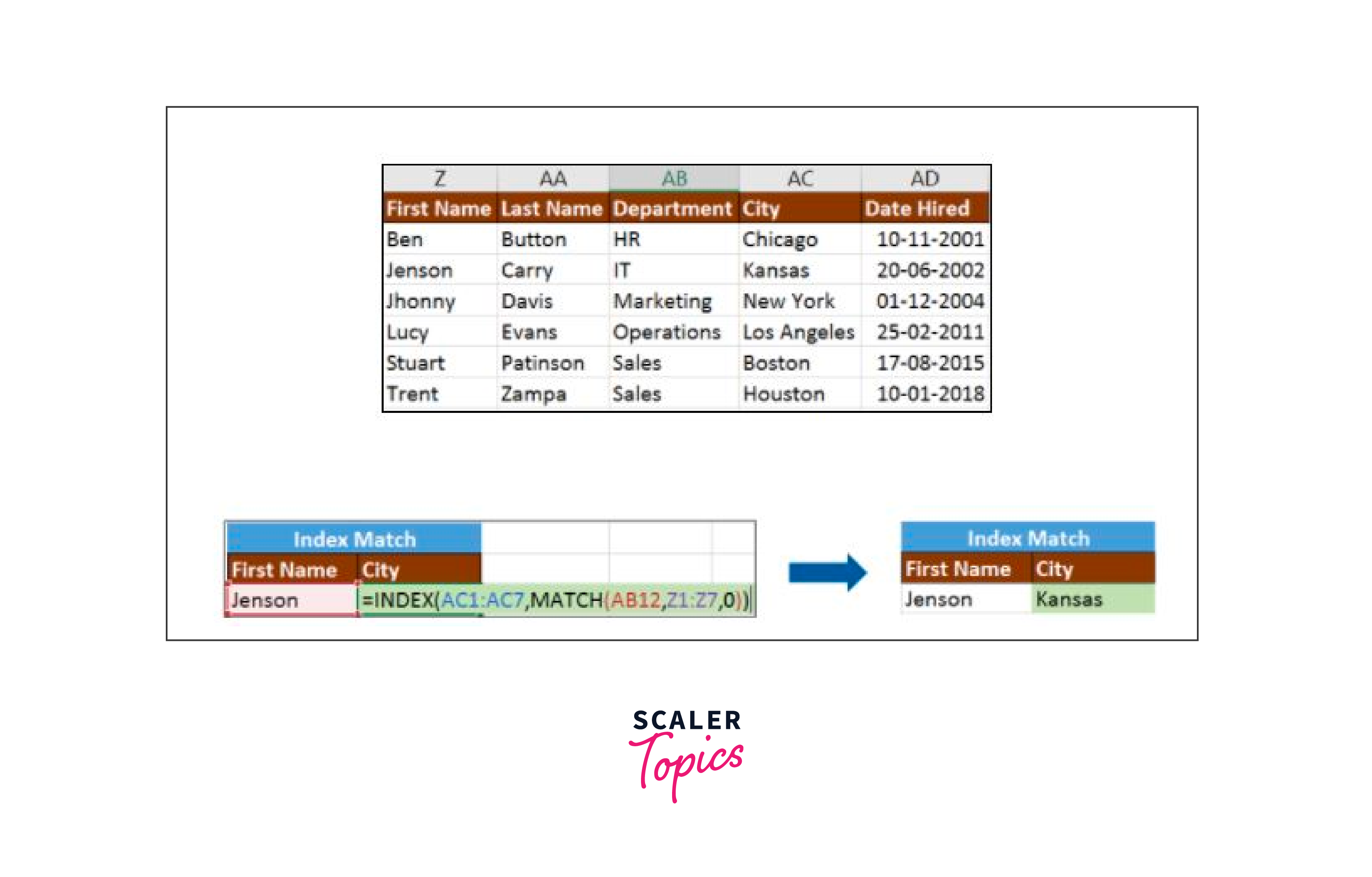
23. INDEX-MATCH

A value in the leftmost column is returned using the INDEX-MATCH function. You are confined to returning an evaluation from a column to the right using VLOOKUP. Index-match should be used instead of VLOOKUP because VLOOKUP requires more processing power than Excel. This is because it must assess the complete table array that you've chosen. Excel simply needs to take the lookup column and the return column into account when using INDEX-MATCH.

Let's locate the city where Jenson lives using the data below.

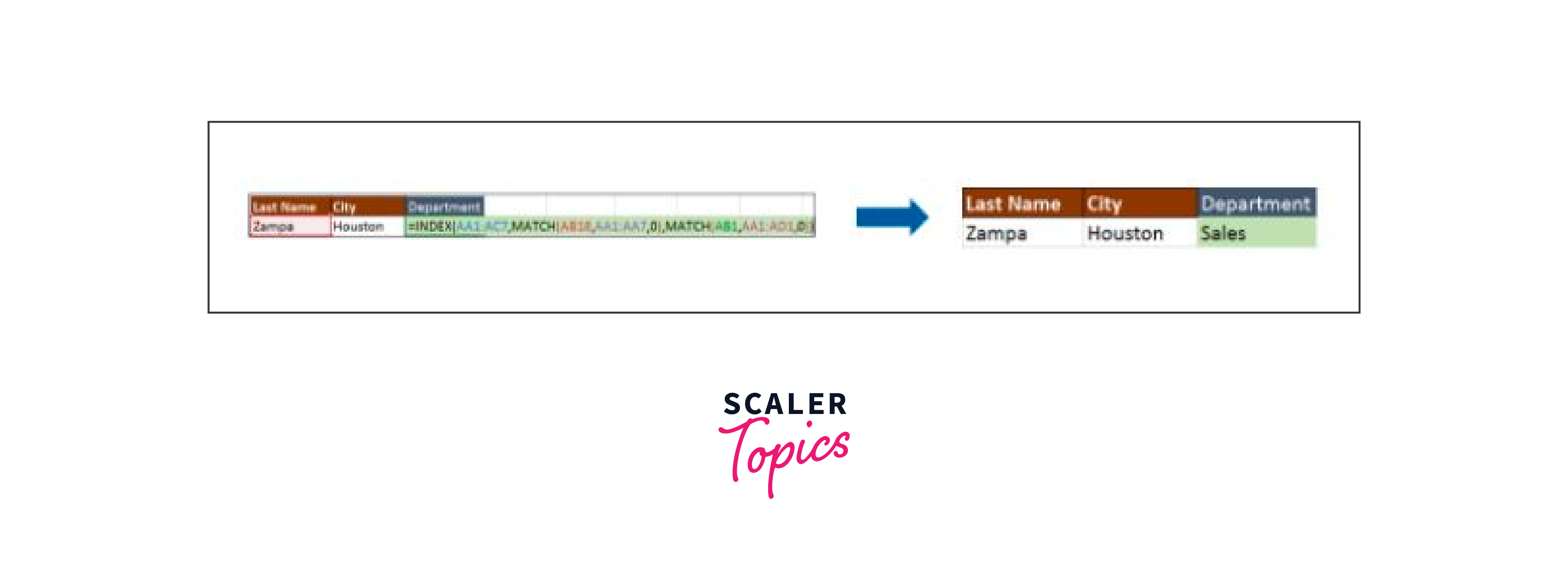
Now let's locate the Zampa section.

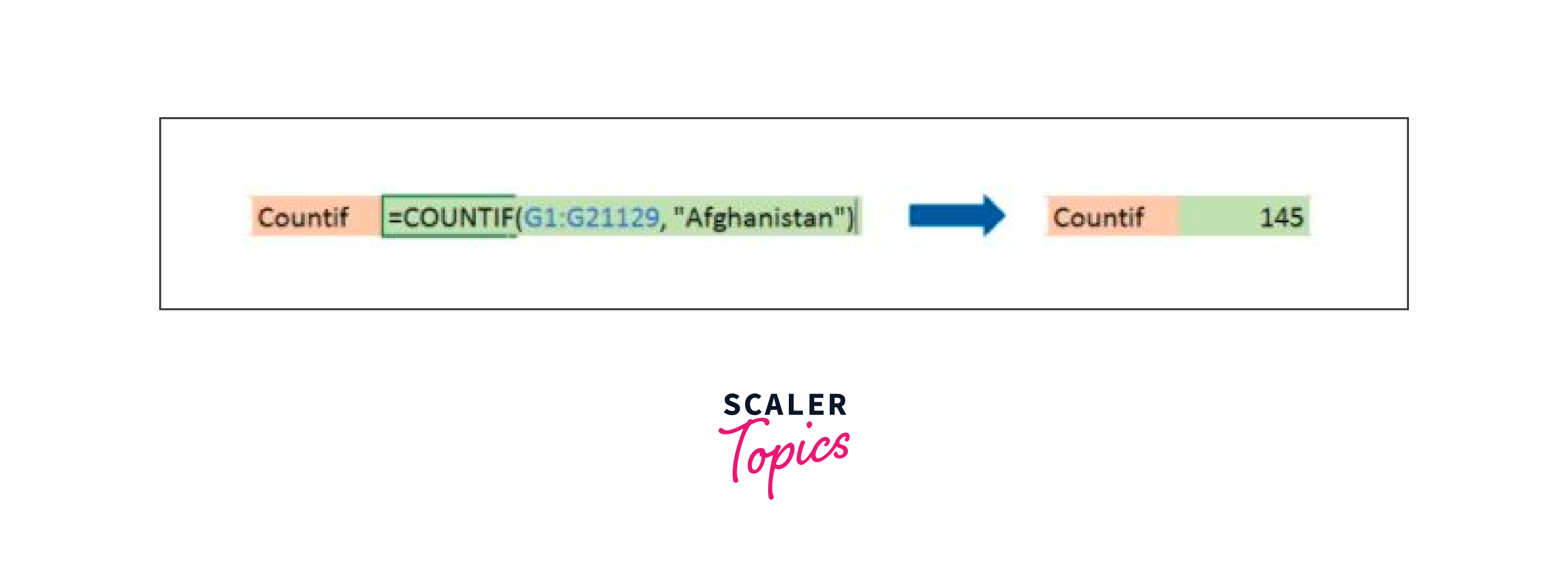
24. COUNTIF

The total number of cells in a range that satisfy the specified condition can be calculated using the function COUNTIF().

A dataset on coronavirus cases and fatalities for each nation and region is provided below.

Let's count the instances in which Afghanistan appears in the table.

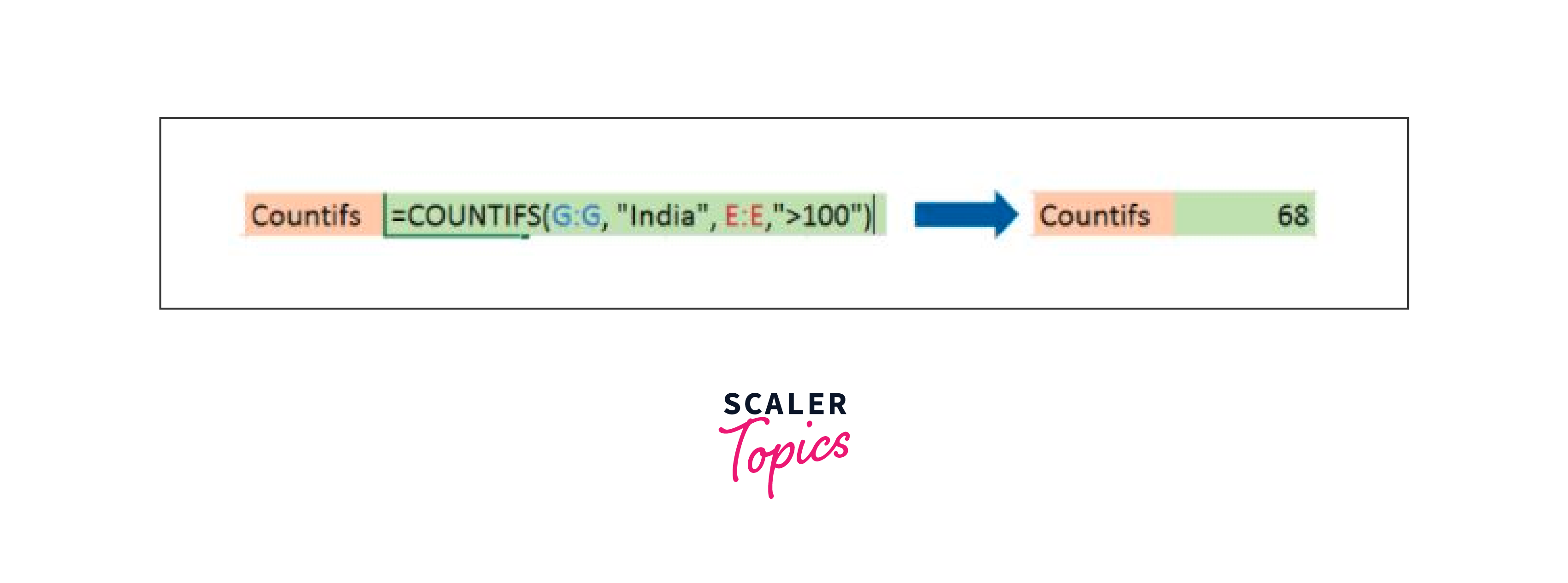
The COUNTIFS function determines how many cells meet a specific set of criteria.

If you wish to calculate the number of days when there were more than 100 instances in India. The COUNTIFS function is used in the following manner.

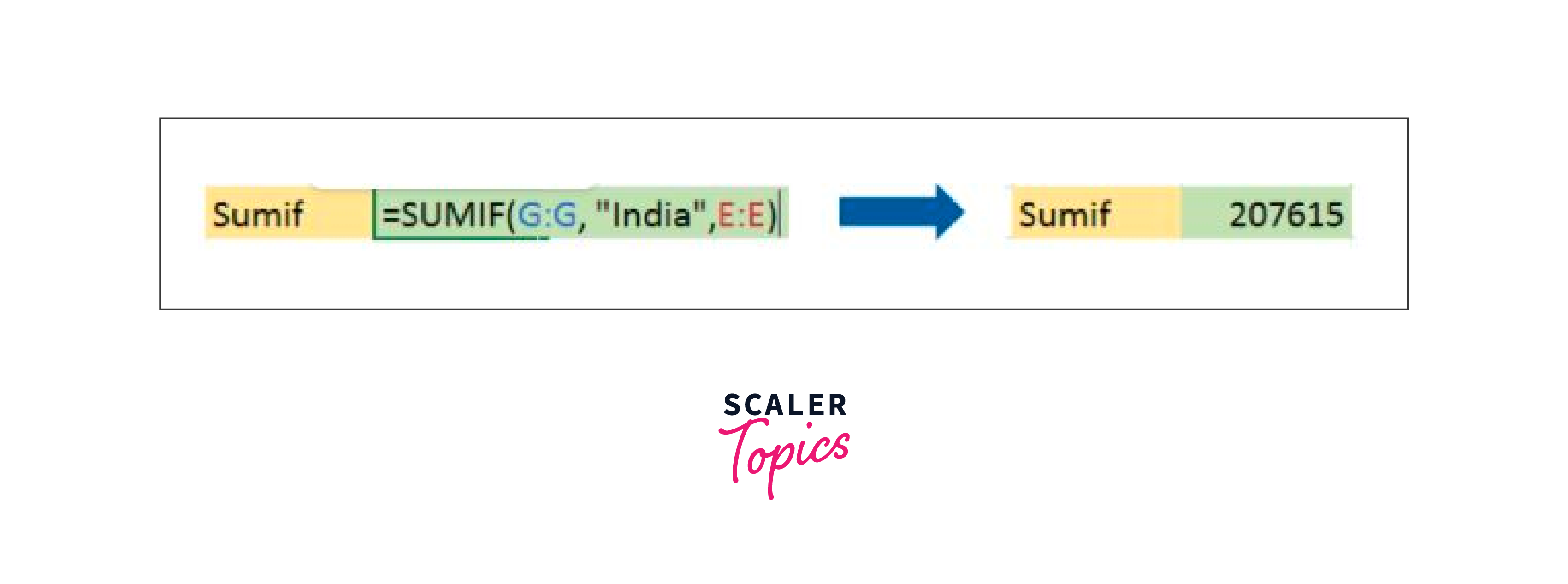
25. SUMIF

The cells indicated by a specific condition or set of criteria are added by the SUMIF() function.

The coronavirus dataset that we will use to determine the overall number of cases in India up until June 3rd, 2020 is provided below. Information in our dataset is available from December 31, 2020, to June 3, 2020.

The cells specified by a certain set of conditions or criteria are added by the SUMIFS() function.