Forecasting in Excel

Why Use Excel in Basic Forecasting?

Excel is an excellent tool for basic forecasting due to its accessibility, ease of use, and robust set of in-built functions. It allows users to quickly identify trends, extrapolate data, and make predictions using methods such as linear regression, moving averages, and exponential smoothing. The FORECAST function and 'What-If Analysis' further simplify the process of predicting future values based on historical data. Its ability to visualize data through charts helps in the easy interpretation of forecasting results. Additionally, Excel's widespread use across industries ensures a high degree of compatibility and makes it a universal choice for basic forecasting tasks.

Create a Forecasting in Excel

You can use historical time-based data to forecast if you have it. When you make a forecasting in Excel, it creates a new worksheet with a table of the past and future values and a chart displaying this information. For example, you can use a forecast to predict upcoming sales, inventory needs, or consumer trends.

1. How to Create a Forecast in Excel?

Two corresponding data series should be entered in a worksheet:

• A collection of timestamps or dates for the timeline
• A collection of values in a sequence
• These figures are projected for upcoming dates.

2. Choose the Two Data Series

The rest of the data is automatically selected by Excel when you select a cell in one of your series.

Click the Forecast Sheet in the Forecast group on the Data tab.

Choose a line or column chart for the forecast's visual representation in the Create Forecast Worksheet box.

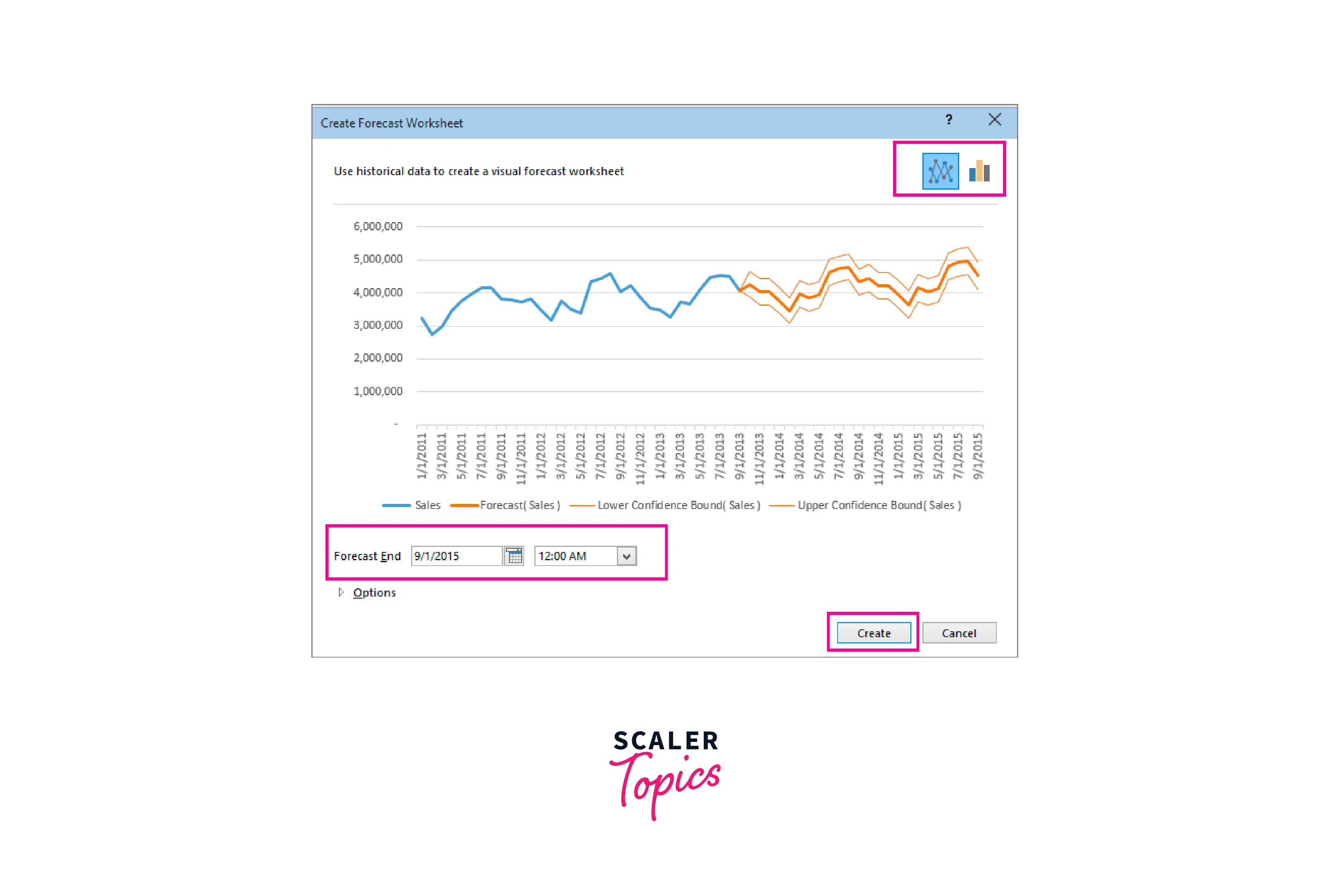
Select a conclusion date in the Forecast End box, then click Create.

Excel creates a new worksheet with a table of the actual and anticipated values and a chart displaying this information.

The new worksheet is located immediately to the left of (or "in front of") the sheet into which you inserted the data series.

Customize your forecast

Click Options to make any forecast-related advanced settings changes.

Forecast Start

Decide when the forecast will start. Only data that existed before the start date are utilized in the prediction when you choose a date earlier than the end of the historical data (this is commonly referred to as "hindcasting").

Confidence Interval

To display or hide Confidence Interval, check or uncheck the box. The Range in which 95% of future points are anticipated to fall, based on the forecast (with normal distribution), is known as the confidence interval. You may determine the prediction's accuracy using the confidence interval. A smaller interval implies more confidence in the prediction for a particular point. The up and down arrows can modify the 95% confidence level set as the default.

Seasonality

Automatic detection of seasonality yields a number indicating the seasonal pattern's length (or several points). For instance, the seasonality in a 12-month sales cycle, with each point denoting a month, is 12. You can override the automatic detection and enter a number by selecting Set Manually.

Timeline Range

The timeline's Range can be modified here. This Range needs to match the Values Range.

Values Range

Here, alter the Range that was used for your value series. This Range must match the Timeline Range exactly.

Fill Missing Points Using

Excel uses interpolation to deal with missing points, which means that if less than 30% of the points are missing, a missing point will be filled in as the weighted average of its neighbors' points. Click Zeros in the list to treat the missing points as zeros instead.

Aggregate Duplicates Using

Excel will take the average of any values in your data with the same timestamp. Select the calculation from the list to use a different method, such as Median or Count.

Include Forecast Statistics

By doing this, statistics are provided by FORECAST.ETS.STAT functions are added to the database. These statistics include the smoothing coefficients (Alpha, Beta, and Gamma) and error metrics (MASE, SMAPE, MAE, and RMSE).

Formulas used in forecasting data

A table with the historical and forecasted data and a chart is produced when you employ a formula to make a forecast. Using your current time-based data with the AAA version of the Exponential Smoothing (ETS) method, the prediction forecasts future values.

The following columns, three of which are computed columns, may be present in the table:

• Time column in the past (your time-based data series)
• (Your related values data series) Historical values column
• Column for forecasted values (estimated with FORECAST.ETS)

The confidence interval is represented by two columns and was calculated using FORECAST.ETS.CONFINT. Only when the Confidence Interval checkbox is selected in the Options section of the box do these columns appear.

Excel FORECAST Functions

Six different forecasting Excel functions are available in the most recent versions of Excel.

These two operations both perform linear forecasts:

• FORECAST is a historical function for Excel 2013 and older that uses linear regression to forecast future values.
• The new suite of forecasting tools in Excel 2016 and Excel 2019 includes the LINEAR function, which is identical to the FORECAST function.

FORECAST

Excel's FORECAST tool uses linear regression to forecast a future value. In other words, FORECAST calculates a value from the past along a line of greatest fit.

The FORECAST function has the following syntax:

Where:

• A numerical x-value for which you want to forecast a new y-value is called X (mandatory).
• Known_y's is an array of known dependent y-values that is necessary.
• Known_x's is an array of independently known x-values.
• All versions of Excel for Office 365, including Excel 2019, Excel 2016, Excel 2013, Excel 2010, Excel 2007, Excel 2003, Excel XP, and Excel 2000, include the FORECAST function.

FORECAST.LINEAR

THE PROJECTION. The FORECAST function's contemporary equivalent is the LINEAR function. The aim and syntax are the same:

The versions of Excel for Office 365, Excel 2019, and Excel 2016 all include this feature.

Both functions employ the linear regression equation to determine the future y-value:

Where the intercept (a constant) is:

And the line's slope, or b coefficient, is:

The x and y values represent the sample means (averages) of the known x and y values, respectively.

Example:

The FORECAST and Excel, as was already explained. The goal of LINEAR functions is to forecast linear trends. Therefore, they are most effective with linear datasets and when you wish to estimate a general trend while disregarding minor data variations.

We'll use our website traffic as an example, attempting to forecast it based on the data from the previous three weeks for the upcoming seven days.

The forecast formula is as follows, using the known y-values (number of visitors) in B2:B22 and the known x-values (dates) in A2:A22.

Excel 2019 - Excel 2000:

Excel 2016 and Excel 2019:

Where A23 is a fresh x-value that you want to forecast a fresh y-value for.

Depending on the version of Excel you are using, enter one of the formulas above in any blank cell in row 23, duplicate it down to however many cells you require, and you will obtain the following result:

Plotted on a graph, our linear forecast looks as follows:

FORECAST.ETS

Forecasts using exponential smoothing are made using the FORECAST.ETS function and are based on several current variables.

The function's name refers to predicting a future value using the AAA implementation of the Exponential Triple Smoothing (ETS) method. This program recognizes seasonality patterns and confidence intervals to smooth out small discrepancies in data trends. The letters "AAA" stand for "additive error, trend, and seasonality."

In Excel for Office 365, Excel 2019, and Excel 2016, the FORECAST.ETS function is accessible.

The Excel FORECAST.ETS has the following syntax:

Where:

The data point to forecast a value for is Target_date (mandatory). It can be expressed as a number or a date/time.

Values is the Range or collection of previous data you wish to forecast future values for.

Timeline: an array of dates, times, or independent numeric values with a predetermined interval between them (needed).

Seasonality (optional): a measure of how long the seasonal pattern lasts:

• Excel uses positive, full numbers to automatically identify seasonality when the value is 1 or omitted (the default).
• 0 indicates a linear forecast with no seasonality.
• The number of hours a year, 8,760, is the maximum amount of seasonality permitted. The #NUM! error will be produced by a greater seasonality number.
• Data completion (optional) fills in the blanks.
• Fill in the missing spots using the average of the nearby points, either 1 or omitted (the default) (linear interpolation).
• 0 - the missing points are treated as zeros.
• Aggregation (optional): Describes how to combine several data items with the same time stamp.
• AVERAGE is used for aggregate if the value is 1 or omitted (the default).
• The following options are also available to you: 2 - COUNT, 3 - COUNTA, 4 - MAX, 5 - MEDIAN, 6 - MIN, and 7 - SUM.

5 things you should know about FORECAST.ETS

• The timeline must have a regular interval for the FORECAST.ETS function to operate correctly, such as hourly, daily, monthly, quarterly, yearly, etc.
• Non-linear data sets with seasonal or recurring patterns best suit this function.
• The function returns to a linear forecast when Excel cannot identify a pattern.
• The function can still use up to 30% of the data points in an incomplete dataset. How the missing points are handled depends on the data completion argument's value.
• There could be duplication in the date/time series, notwithstanding the requirement for a timeline with a consistent step. The aggregation option specifies how to aggregate data that have the same timestamp.

Example

Let's create a FORECAST.ETS formula using the same data set as in the preceding example to demonstrate how the future values predicted by exponential smoothing differ from those predicted by linear regression:

Where:

• The target date is A23.
• $B$2: $B The past data (values) are $22.
• $A$2: $A The dates (timeline) are $22.

We rely on Excel defaults by leaving out the final three inputs (seasonality, data completion, or aggregation). And Excel accurately predicts the trend.

FORECAST.ETS.CONFINT

A forecasted value's confidence interval is determined using the FORECAST.ETS.CONFINT function.

The confidence interval can be considered a gauge of a forecast's accuracy. The forecast is more certain for a given data point when the interval is smaller.

Available in Excel for Office 365, Excel 2019, and Excel 2016 is the FORECAST.ETS.CONFINT.

The function's arguments are as follows:

As you can see, FORECAST.ETS.CONFINT's syntax is similar to that of the FORECAST.ETS function except for the following extra argument:

• Specifies the confidence level in the estimated interval with a value between 0 and 1. Confidence_level is optional. Although percentages are also acceptable, it is typically provided as a decimal figure. For instance, write 0.9 or 90% to specify a 90% confidence level.
• If left blank, a projected data point is assumed to fall inside this Range 95% of the time from the value supplied by FORECAST.ETS. If not, the default value of 95% is used.
• The formula returns the #NUM! error if the confidence level is outside the supported Range (0-1).

Example

Let's calculate the confidence interval for our test data set to show how it works in practice:

Where:

• The target date is A23.
• $B$2: $B The historical data is $22.
• $A$2: $A The dates are $22.

To instruct Excel to utilize the default choices, the final four arguments are omitted:

• Decide on a 95% confidence level.
• automated detection of seasonality.
• Fill in the gaps using the average of the surrounding points.
• Make use of the AVERAGE function to combine various data values with the same date.

Please look at the screenshot below (some rows with historical data are omitted for space reasons) to better understand what the returned values imply.

The outcome of the formula in D23 is 6441.22 (rounded to two decimal places). It means that the prediction for 11-Mar should, in 95% of cases, be within 6441.22 of the predicted value of 61,075 (C3). This equates to 61,075 ± 6441.22.

You can compute the confidence interval boundaries for each data point to determine the Range in which the predicted values will likely fall.

Subtract the confidence interval from the anticipated value to obtain the lower bound:

Add the confidence interval to the predicted value to obtain the upper bound:

Where D23 is the confidence interval produced by FORECAST.ETS.CONFINT and C23 is the anticipated value returned by FORECAST.ETS.

You can easily see the expected values and the confidence interval if you copy down the above calculations and plot the results on a chart:

FORECAST.ETS.SEASONALITY

The length of an ongoing pattern in the given timeline is determined using the FORECAST.ETS.SEASONALITY function. Because both functions employ the same algorithm to identify seasonality, they are closely related to FORECAST.ETS.

The versions of Excel for Office 365, Excel 2019, and Excel 2016 all include this feature.

The following is the syntax for FORECAST.ETS.SEASONALITY:

The formula looks like this for our data set:

The seasonality 7 is returned, perfectly matching the weekly trend on our historical data.

FORECAST.ETS.STAT

The FORECAST returns a specified statistical value about a time series exponential smoothing forecast.ETS.STAT function.

It is accessible in Excel for Office 365, Excel 2019, and Excel 2016, much like other ETS functions.

The function's syntax is as follows:

Which statistical value to return is specified by the statistic_type argument:

The smoothing value between 0 and 1 known as alpha (base value) determines how much each data point is weighted. Recent data is given greater weight the higher the value. The variable between 0 and 1 that governs how to calculate trends is called beta (trend value). Recent trends are given more weight the higher the value.

Gamma (seasonality value), a number between 0 and 1, determines how seasonal the ETS forecast will be. The recent seasonal period is given more weight the higher the value.

MASE (mean absolute scaled error) is a metric for gauging the accuracy of forecasts. A measure of accuracy based on absolute or relative mistakes is called SMAPE (symmetric mean absolute percentage error).

Measuring the average magnitude of prediction mistakes, regardless of their direction, is called MAE (mean absolute error).

Root mean square error, or RMSE, is a metric for comparing anticipated and actual values. the step size that was discovered in the timeline.

For instance, we can use the following formula to return the Alpha parameter for our sample data Set:

The algorithms for additional statistical values are displayed in the screenshot below: