Graph Representation in Data Structure

Graphs, as non-linear data structures comprising nodes and edges, represent relationships between entities. Three classic graph representation in data structure include Adjacency Matrix, Adjacency List, and Incidence Matrix. While Adjacency Matrix offers fast edge retrieval but consumes more space, Adjacency List is space-efficient but slower for edge retrieval. Incidence Matrix is rarely used due to its inefficient space utilization and slower edge retrieval compared to the other two graph representations.
Representations of Graph in Data Structure
The three common ways to represent a graph are :
- Adjacency Matrix
- Incidence Matrix
- Adjacency List
Adjacency Matrix
As the name suggests, the adjacency matrix is a matrix representation of a graph. What does the word 'adjacency' mean here? We use this word since this matrix is used to mark the nodes in the graph that are 'adjacent' or directly connected by an edge (if the graph is undirected). If the graph is directed, then the matrix is used to mark the nodes in the graph that are pointed to by other nodes. Now how is this done?
Let's say we have an undirected graph like this:

This is a very simple graph, that has 5 nodes - A, B, C, D, E. Let's also make a note of all the existing edges in the graph - AB, BA, AC, CA, BC, CB, BE, EB, CD, DC, DE, ED. Now, to represent this graph in the form of an adjacency matrix, we're going to create a matrix of size n * n where n is the number of nodes in the graph. The matrix graph[][] is going to represent our graph with graph[i][j] having a value of 1 if an edge between the vertex i and vertex j (or from vertex i to vertex j in case of a directed graph) exists and 0 otherwise. For weighted graphs, however, the value at graph[i][j] for an existing edge is equal to the weight of that edge. Now here, we must fill in the value at graph[i][j] as well as graph[j][i] in the case of an undirected graph.
The representation of the graph in the example above would look like this:
| A | B | C | D | E | |
|---|---|---|---|---|---|
| A | 0 | 1 | 1 | 0 | 0 |
| B | 1 | 0 | 1 | 0 | 1 |
| C | 1 | 1 | 0 | 1 | 0 |
| D | 0 | 0 | 1 | 0 | 1 |
| E | 0 | 1 | 0 | 1 | 0 |
As you can see in this matrix, we have the columns and rows representing each vertex, and wherever an edge exists, we have a value = 1, and a value = 0 where an edge does not exist.
For a directed graph,
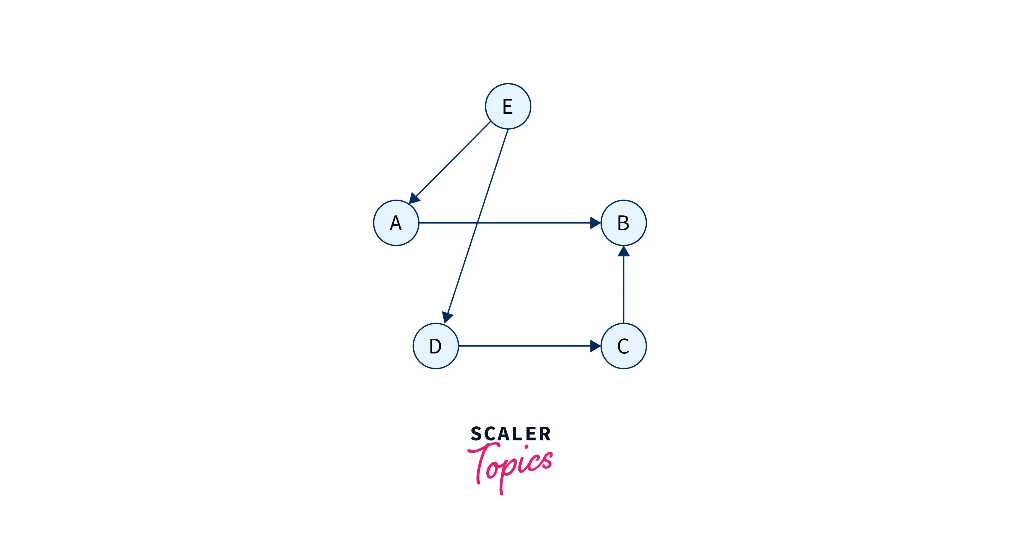
The adjacency matrix would have looked like this.
| A | B | C | D | E | |
|---|---|---|---|---|---|
| A | 0 | 1 | 0 | 0 | 0 |
| B | 0 | 0 | 0 | 0 | 0 |
| C | 0 | 1 | 0 | 0 | 0 |
| D | 0 | 0 | 1 | 0 | 0 |
| E | 1 | 0 | 0 | 1 | 0 |
Let us now look at the pros and cons of this representation of a graph.
Pros
- Easy to implement, follow and visualize.
- Removal of an edge from the graph takes O(1) time since we simply have to change a value in the matrix.
- Queries about edges in the graph from a node u -> v can also be done in O(1) time since accessing a value from the matrix takes O(1) time.
Cons
- Since this representation of a graph is a sparse matrix (a matrix with more values as 0 than other values), it consumes a lot of space. The space taken by this graph is $O(V^2)$ where V is the number of vertices/nodes in the graph.
- Adding a vertex to this graph would take O(V2) time.
- If you would like to compute the neighbors of a particular vertex, it would take O(V) time which is not efficient.
Incidence Matrix
Another matrix representation of the graph is the incidence matrix representation. Of course, since it is a matrix it is also initialized as an array of arrays graph[][] where graph[i][j] would represent an edge. However, here, there's a small difference. The matrix size would not be V x V (V = number of vertices). It would instead be V x E i.e. a matrix with rows as the vertices and columns as edges.
This representation of graphs is usually used for graphs that are directed. If there is an outward edge E1 from node/vertex A, then the value at graph[A][E1] would be 1. If there is an inward edge E1 to node B, then the value at graph[B][E1] would be -1.
For a graph that looks like this:
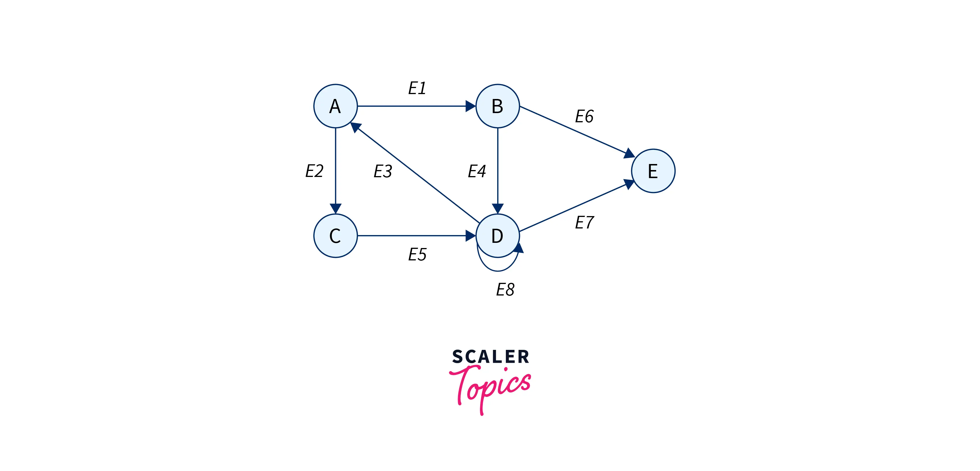
with nodes - A, B, C, D, E and edges E1, E2, E3, E4, E5, E6, E7, E8, the incidence matrix would look like this:
| E1 | E2 | E3 | E4 | E5 | E6 | E7 | E8 | |
|---|---|---|---|---|---|---|---|---|
| A | 1 | 1 | -1 | 0 | 0 | 0 | 0 | 0 |
| B | -1 | 0 | 0 | 1 | 0 | 1 | 0 | 0 |
| C | 0 | -1 | 0 | 0 | 1 | 0 | 0 | 0 |
| D | 0 | 0 | 1 | -1 | -1 | 0 | 1 | 1 |
| E | 0 | 0 | 0 | 0 | 0 | -1 | -1 | 0 |
To understand this matrix, look at it column by column, i.e. for every edge. There are just 3 possible values -- 0, 1, -1. If the value is 0, it means that this particular edge is not received by this node (the row value), or it is not originating from this node either. If the value is 1, it means that this edge (the column) originates from the node (row value). Likewise, if the value is -1, the edge is received by the node.
Let's now discuss the pros and cons of this representation.
Pros
- The matrix takes just O(E) time to build where E is the number of edges.
Cons
- This graph representation in data structure has more space complexity than other representations of graphs.
Adjacency List
Both the approaches that we saw prior to this one, represented a graph using a matrix. However, this representation makes use of an array of linked lists to store the graph. Let's see how.
We have an initial array or a list, that stores all the vertices, i.e. an array of size equal to the number of vertices in our graph. These elements of the array are also the heads of multiple linked lists. The heads point to the next element that they share an edge within the case of an undirected graph, and in the case of a directed graph, the linked list consists of all the vertices that the head vertex points to. So, a graph like:
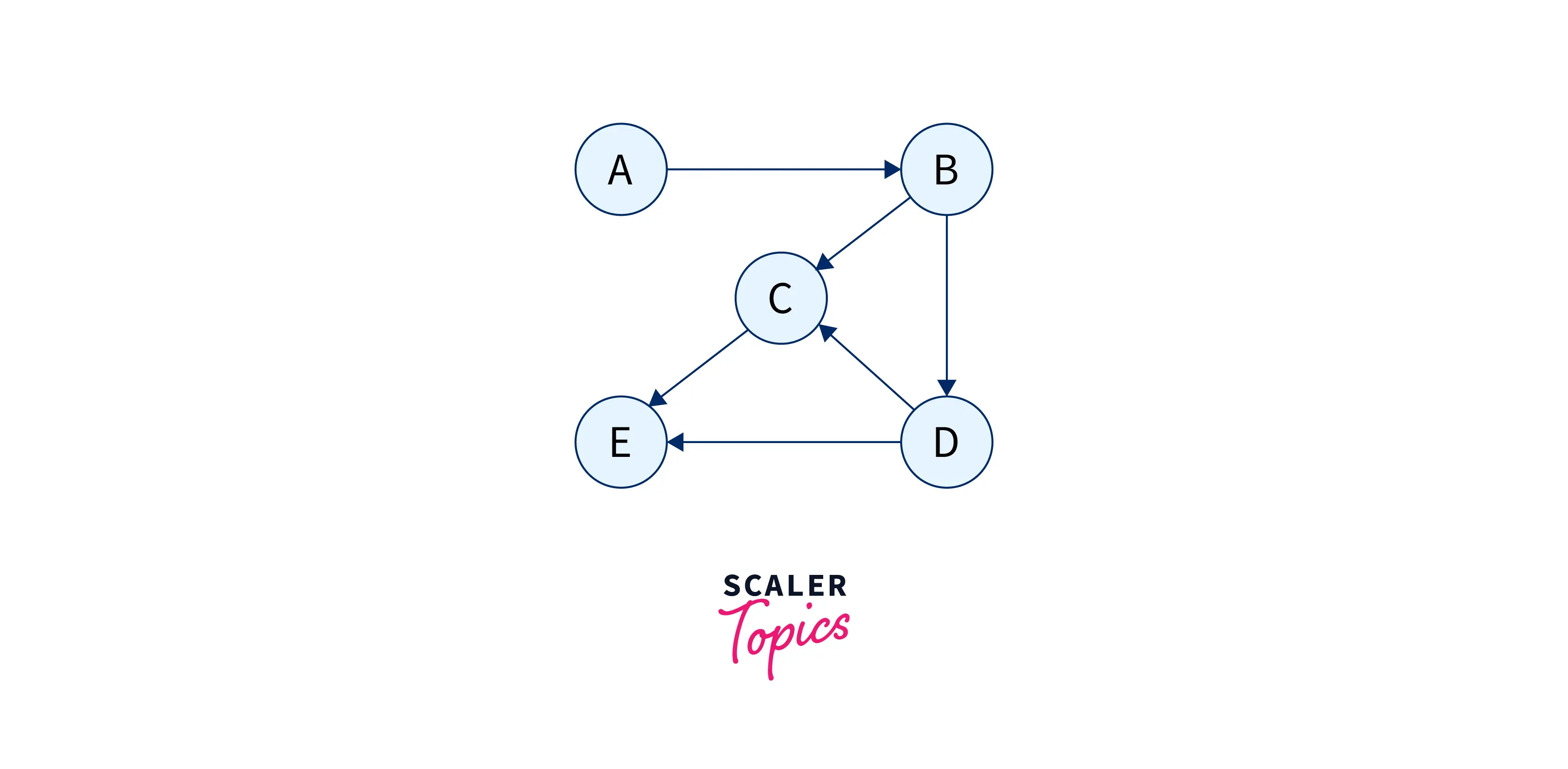
looks like this when represented in the form of an adjacency list:
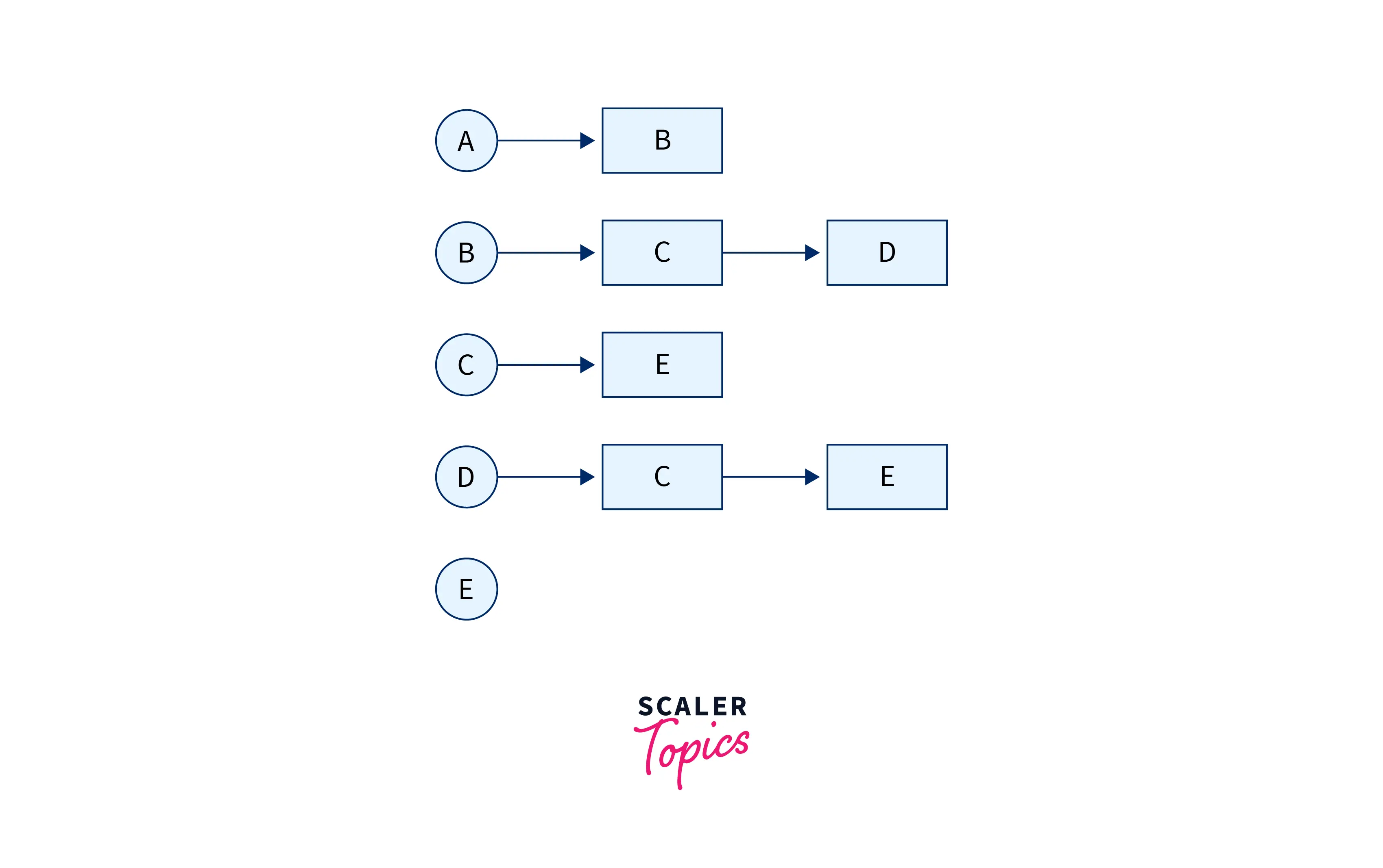
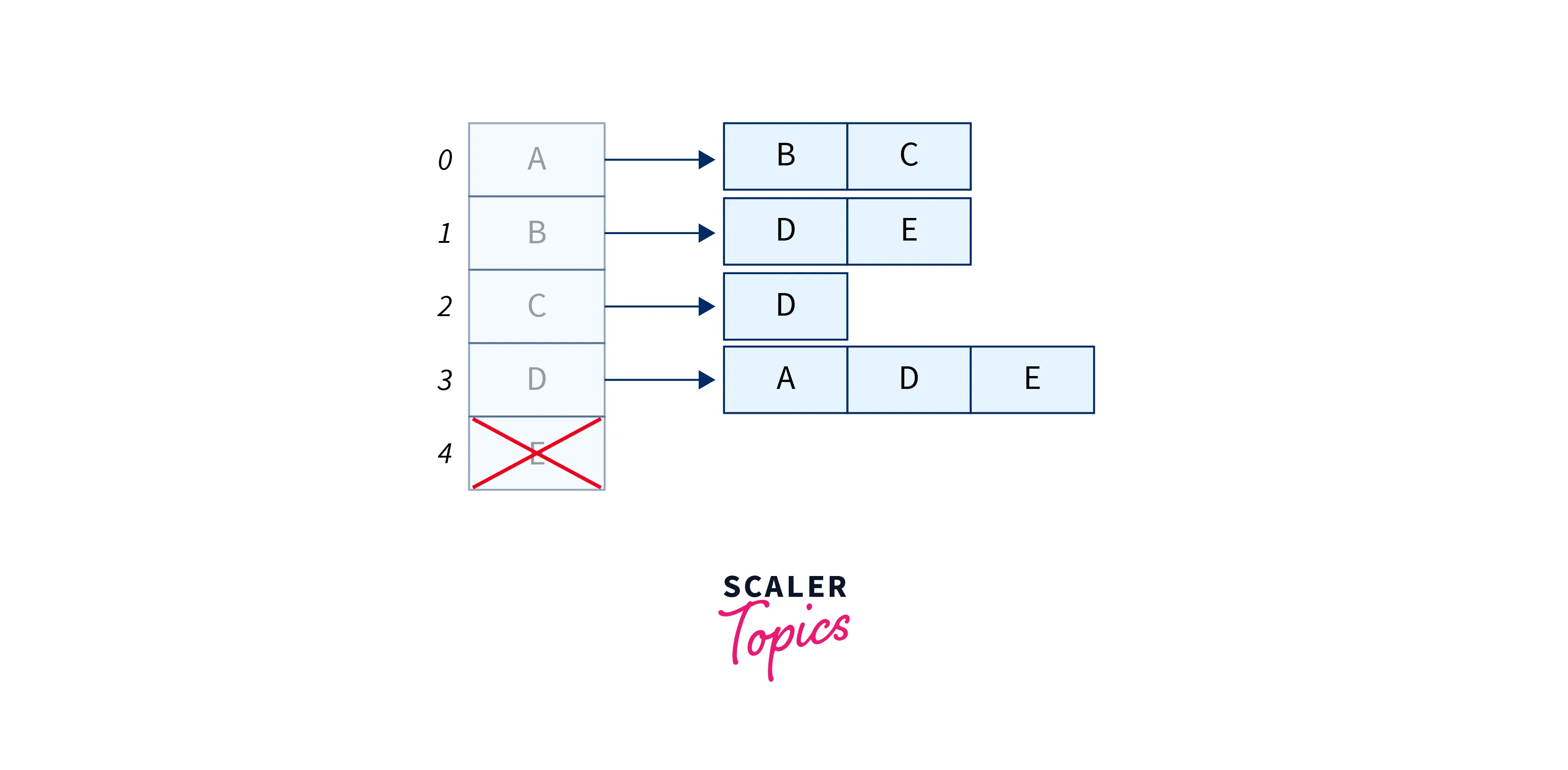
Another way to represent a graph using an adjacency list is to have an array of vertices that are also the heads of the linked lists. These heads point to arrays that contain all the nodes that are "adjacent" to it in the form of a list, like this:
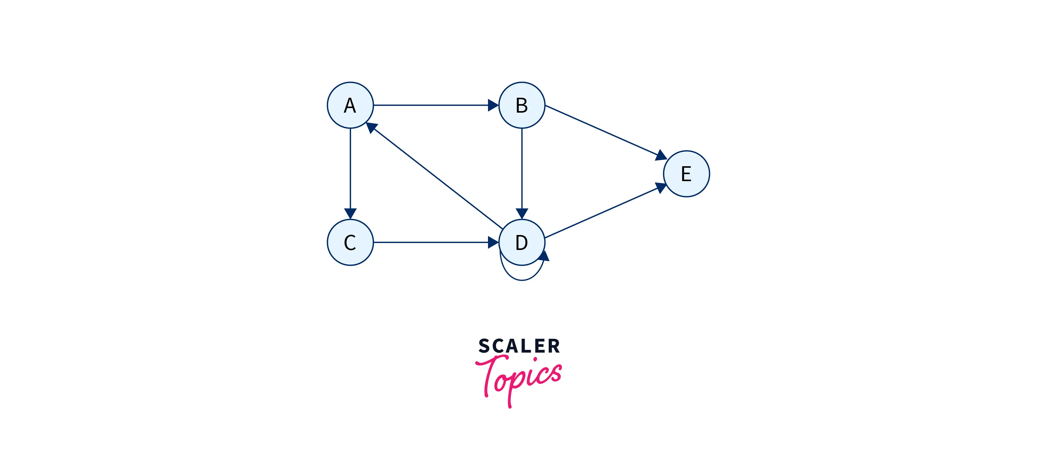
For a graph as above, the adjacency list representation can also look like this:
For an undirected graph as below:
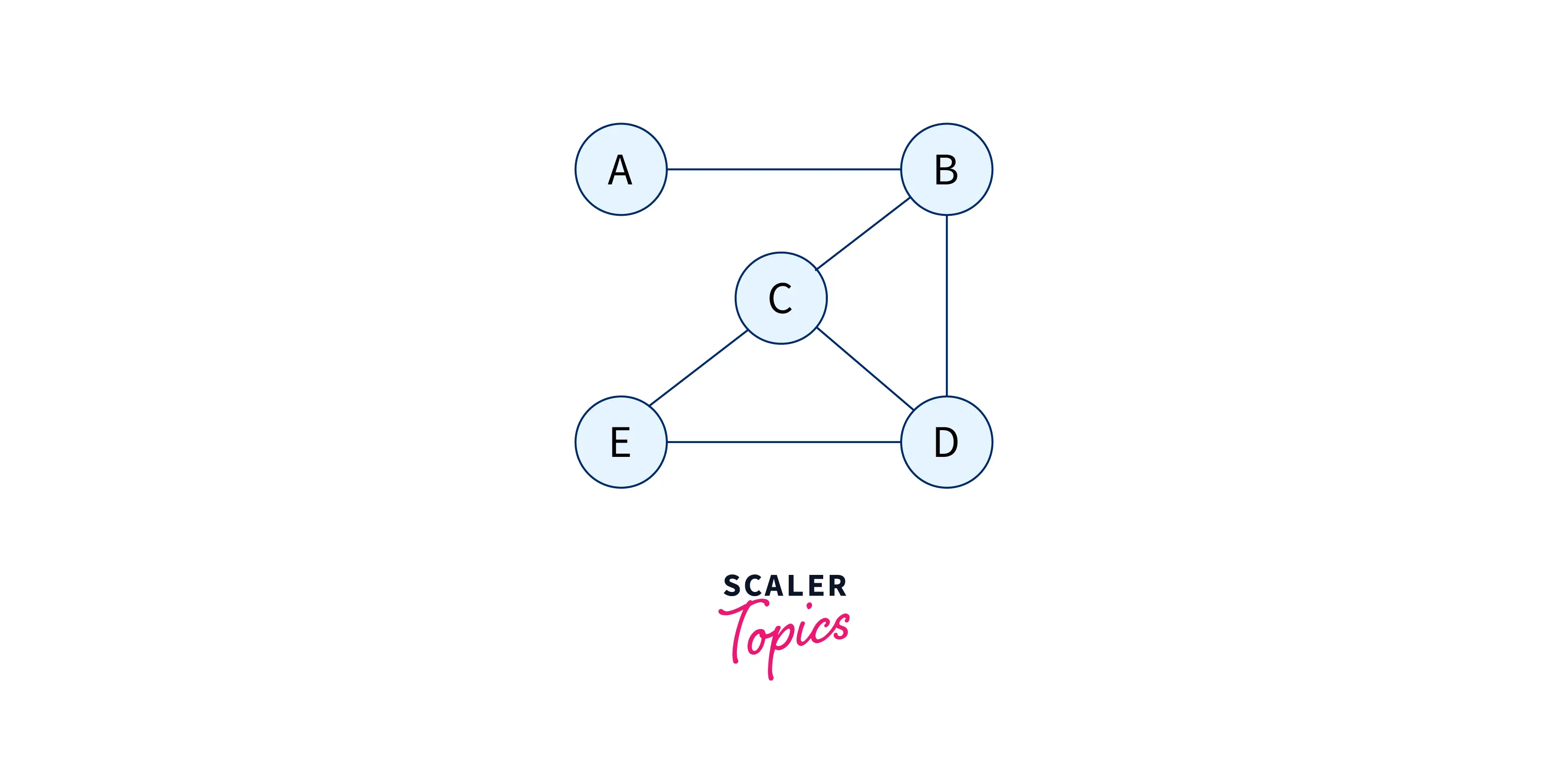
We can have an adjacency list that looks like this:
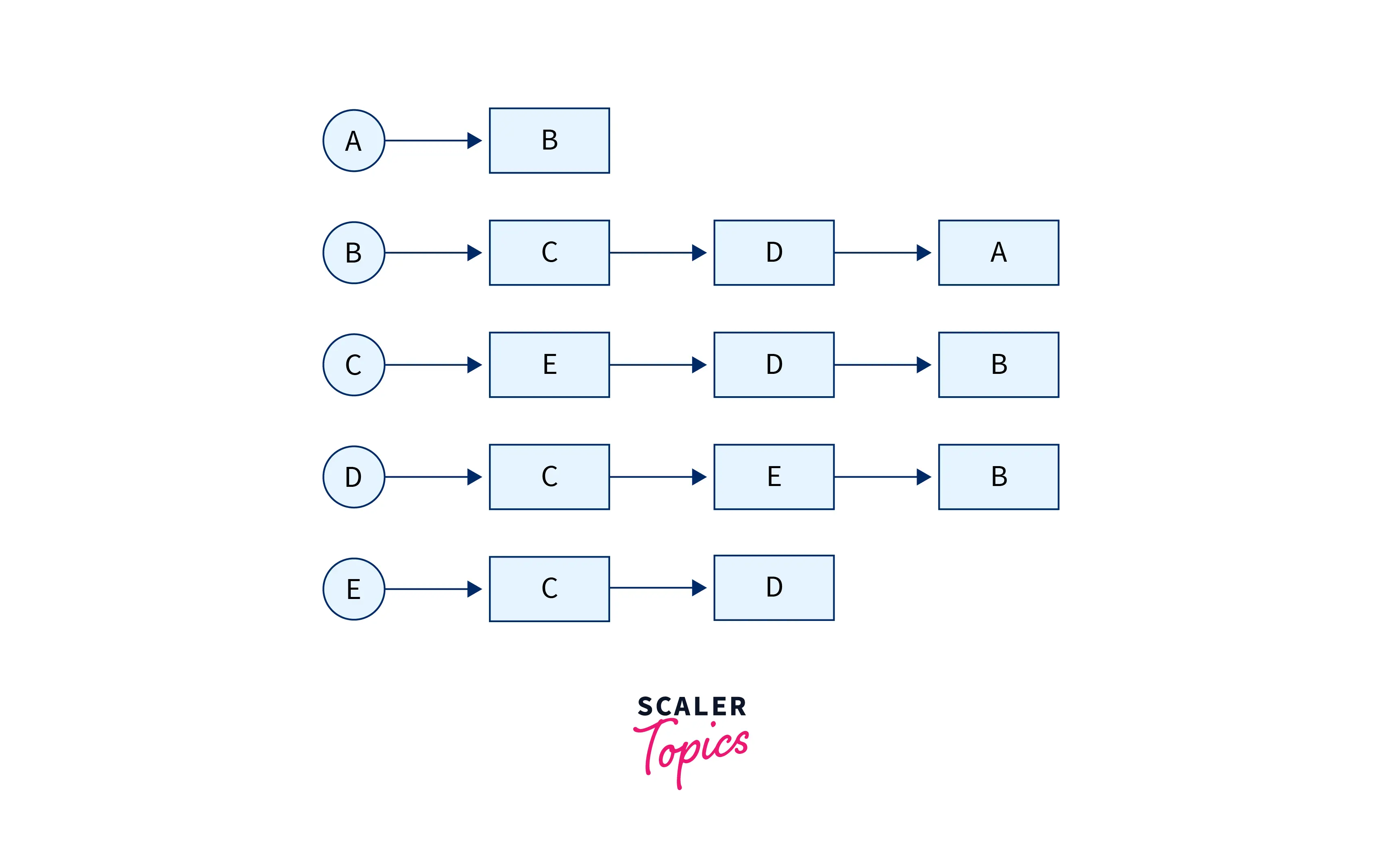
Now coming on to the pros and cons of the adjacency list representation of a graph.
Pros
- This representation of a graph saves a lot of space which is O(V + E) since we are not using matrices, which are usually sparse and consume a lot of space.
- The adjacency list representation enables us to search for an edge faster when compared to the adjacency matrix representation.
Cons
- Not the best representation in terms of insertion and deletion of nodes. Deletion, for example, would involve linear search in all linked lists.
Conclusion
- Graphs are fundamental data structures for modeling relationships between entities, with various real-world applications like maps, networks, and social media.
- The three classic representations of graphs in data structures—Adjacency Matrix, Adjacency List, and Incidence Matrix—each offer distinct advantages and disadvantages.
- Each graph representation has its pros and cons, including considerations for space complexity, edge retrieval efficiency, and insertion/deletion operations.
- The choice of graph representation depends on specific application requirements, such as space constraints, frequency of edge retrieval, and dynamic graph changes.
Learn more
To learn more about graphs, refer to this article by scaler topics.
