Hamiltonian Graph

What is Hamiltonian graph?

A Hamiltonian graph $G$ having $N$ vertices and $E$ edges is a connected graph that has a Hamiltonian cycle in it where a Hamiltonian cycle is a closed path that visits each vertex of graph $G$ exactly once.

For example:

The graph above is a Hamiltonian graph because it contains a Hamiltonian path 1-2-4-5-3. To read more about Hamiltonian paths read Hamiltonian path

Properties of Hamiltonian graph:

1. NP-Completeness: Detecting a Hamiltonian path in a given graph is an NP complete problem i.e. we can use either backtracking or guesswork to find the solution.

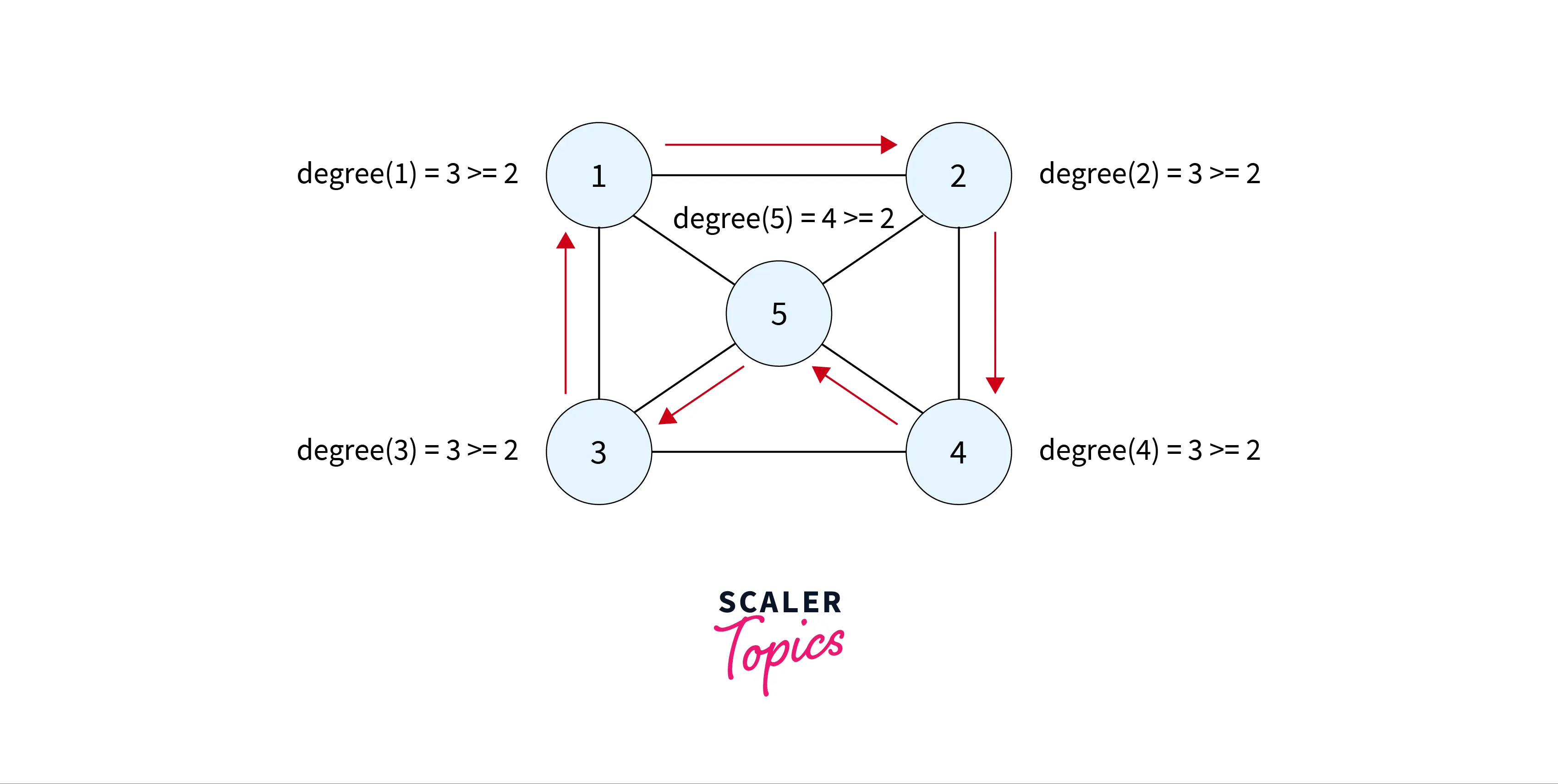
2. Dirac's Theorem: It states that if $G$ is a connected graph having $N$ vertices and $E$ edges, where $N>=3$, then if each vertex $v$ has degree at least $N/2$ i.e. $degree(v) >= N/2$, then $G$ is a Hamiltonian graph. For example, it can be proved for the above graph.

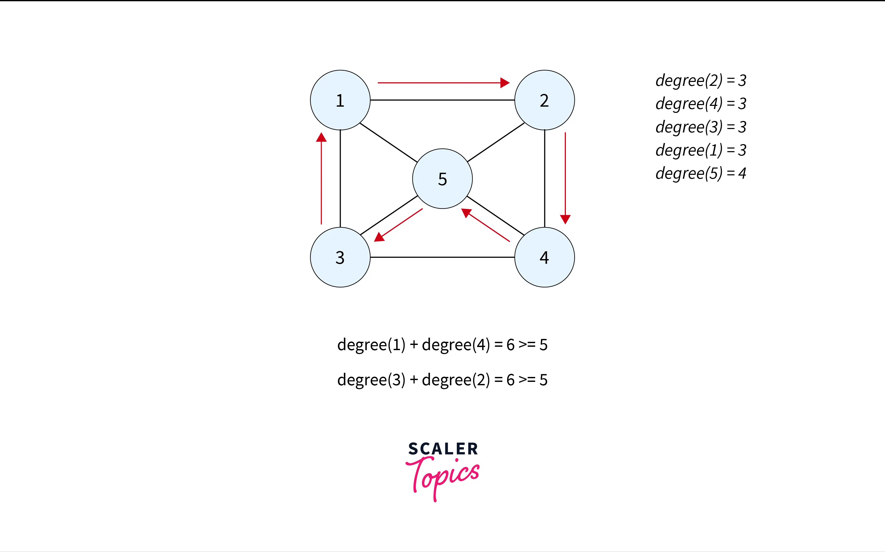
3. Ore's Theorem: It states that if $G$ is a connected graph having $N$ vertices and $E$ edges, where $N>=2$, then if the sum of degrees of any two non-adjacent vertices is at least $N$, then graph $G$ is Hamiltonian Graph. For example, it can be proved for the above graph.

Let's see a program to check for a Hamiltonian graph:

Program to check for a Hamiltonian Cycle

A Hamiltonian graph is a connected graph that contains a Hamiltonian cycle/circuit.

Hamiltonian cycle: Hamiltonian cycle is a path that visits each and every vertex exactly once and goes back to starting vertex.

To check for a Hamiltonian cycle in a graph, we have two approaches. The first approach is the Brute-force approach and the second one is to use Backtracking, Let's discuss them one by one.

Naive-Approach:

The Brute-force way to check for the Hamiltonian cycle is to generate all configurations of the vertices and for each configuration check if it is a valid Hamiltonian cycle.

Consider a predicate function check_Hamiltonian_cycle() which takes the graph in the form of adjacency matrix $adj[][]$ and number of vertices $N$ as arguments and returns if there exists a Hamiltonian cycle.

The Pseudo-code implementation is as follows:

The C++ implementation of the above Pseudo-code is as follows:

Output:

In the above Pseudo-code implementation get_next_permutation() function takes the current permutation and generates the lexicographically next permutation.

Let's understand the time and space complexity:

Time Complexity: The program uses the get_next_permutation() function to generate all permutations while this function has the time complexity of $O(N)$ and for each permutation, we check if this is a Hamiltonian cycle or not and there are total $N!$ permutations. Hence, the overall complexity becomes $O(N! * N)$.

Space Complexity: The program uses a permutation array p of length $N$ as an auxiliary space to check for the cycle, Hence, the space complexity is $O(N)$.

Backtracking Approach:

In this approach, we start from the vertex 0 and add it as the starting of the cycle. Now, for the next node to be added after 0, we try all the nodes except 0 which are adjacent to 0, and recursively repeat the procedure for each added node until all nodes are covered where we check whether the last node is adjacent to the first or not if it is adjacent to the first we declare it to be a Hamiltonian path else we reject this configuration.

Let's see the implementation:

Output:

Time Complexity: The backtracking algorithm basically checks all of the remaining vertices in each recursive call. In each recursive call, the branching factor decreases by one because one node is included in the path for each call.

The time complexity is given by $T(N) = N*(T(N-1)+O(1))$ $T(N) = N*(N-1)* (N-2)*.. = O(N!)$ Therefore, the time complexity is $O(N!)$.

Space Complexity: Since, the algorithm does not use any extra auxiliary space, the space complexity is $O(1)$.

Applications of Hamiltonian graphs

1. Travelling Salesmen Problem: The Travelling salesman problem which asks for the shortest path that a salesperson must take to visit all cities of a given set. This problem actually reduces to finding the Hamiltonian circuit in the Hamiltonian graph such that the sum of the weights of the edges is minimum. To read more about TSP read Travelling Salesman Problem.

2. Optimal Path Calculation: Applications involving paths that visit each intersection(node) of the city exactly once can be solved using Hamiltonian paths in Hamiltonian graphs.

3. Mapping Genomes: Applications involving genetic manipulation like finding genomic sequence is done using Hamiltonian paths. Genomic sequence is made up of tiny fragments of genetic code called reads and it is built by calculating the hamiltonian path in the network of these reads where each read is considered a node and the overlap between two reads as edge.

4. They are used in fields like Computer Graphics, electronic circuit design and operations research.

Check for the Hamiltonian graph

To check whether a given graph is a Hamiltonian graph or not, we need to check for the presence of the Hamiltonian cycle in it, if there exists a Hamiltonian cycle then the graph is called a Hamiltonian graph. Also, the graph must satisfy the Dirac's and Ore's Theorem.

Example of Hamiltonian graph

Let's see and understand an example of a Hamiltonian graph: The hamiltonian graph must satisfy all of the properties mentioned in the definition section of the article.

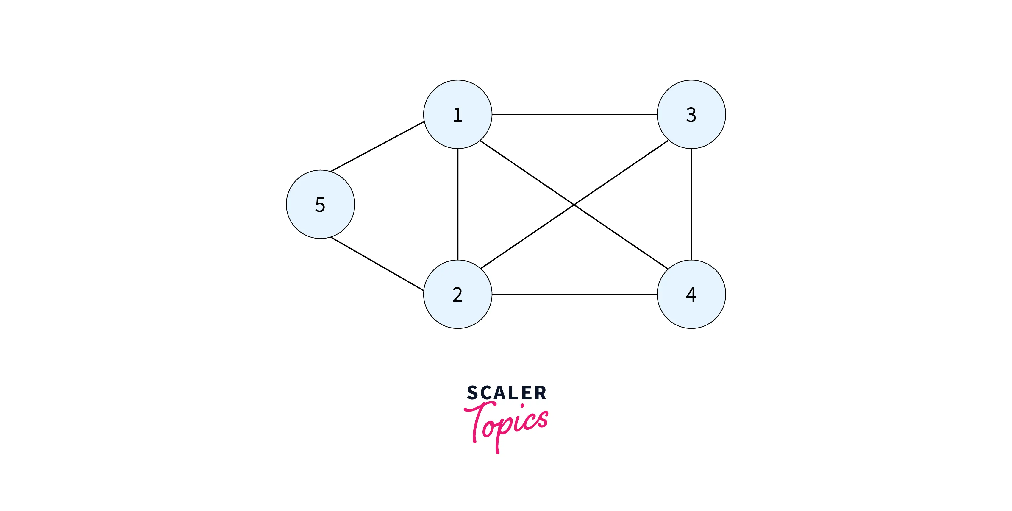
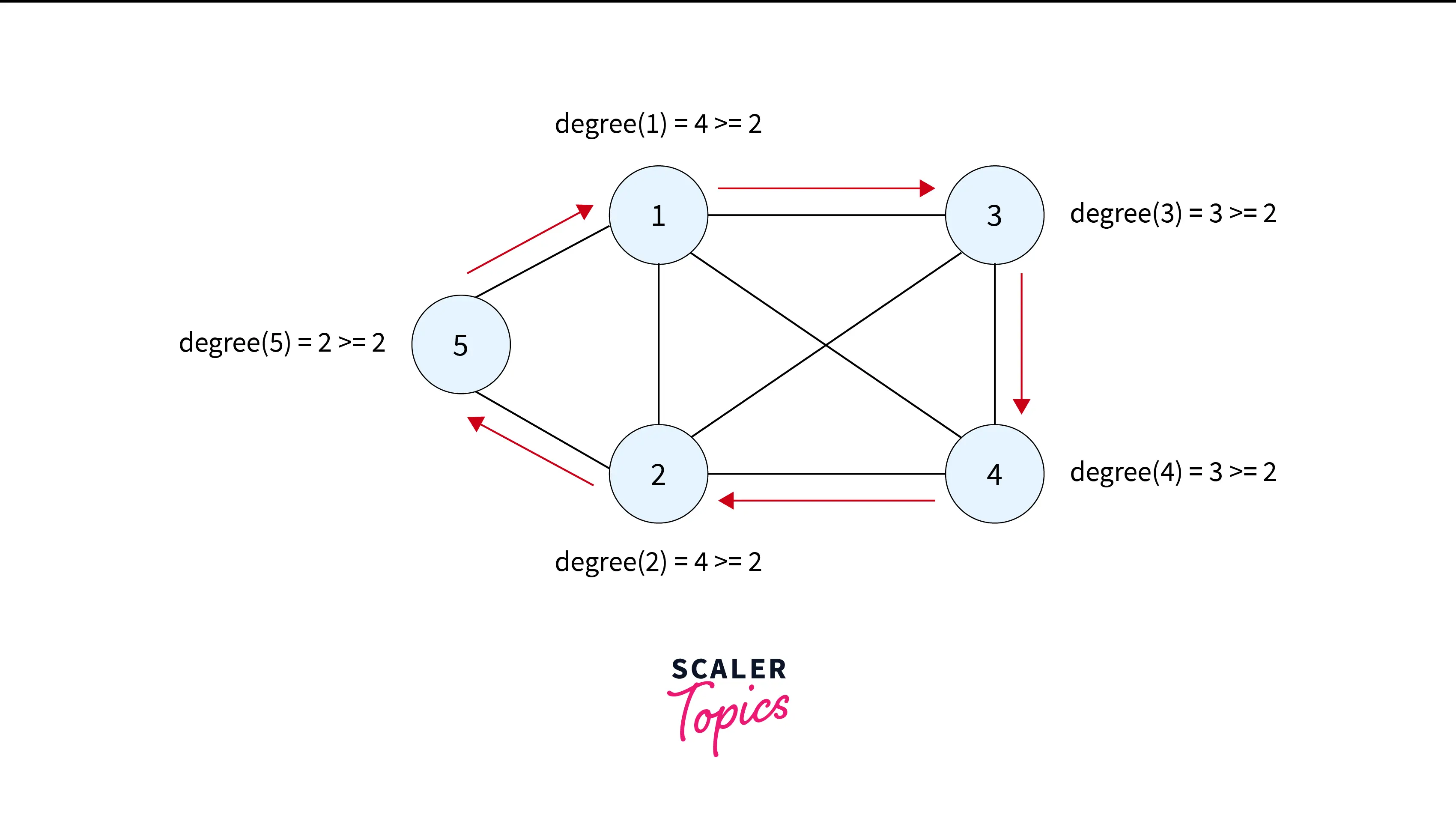
The above figure represents a Hamiltonian graph and the corresponding Hamiltonian path is represented below:

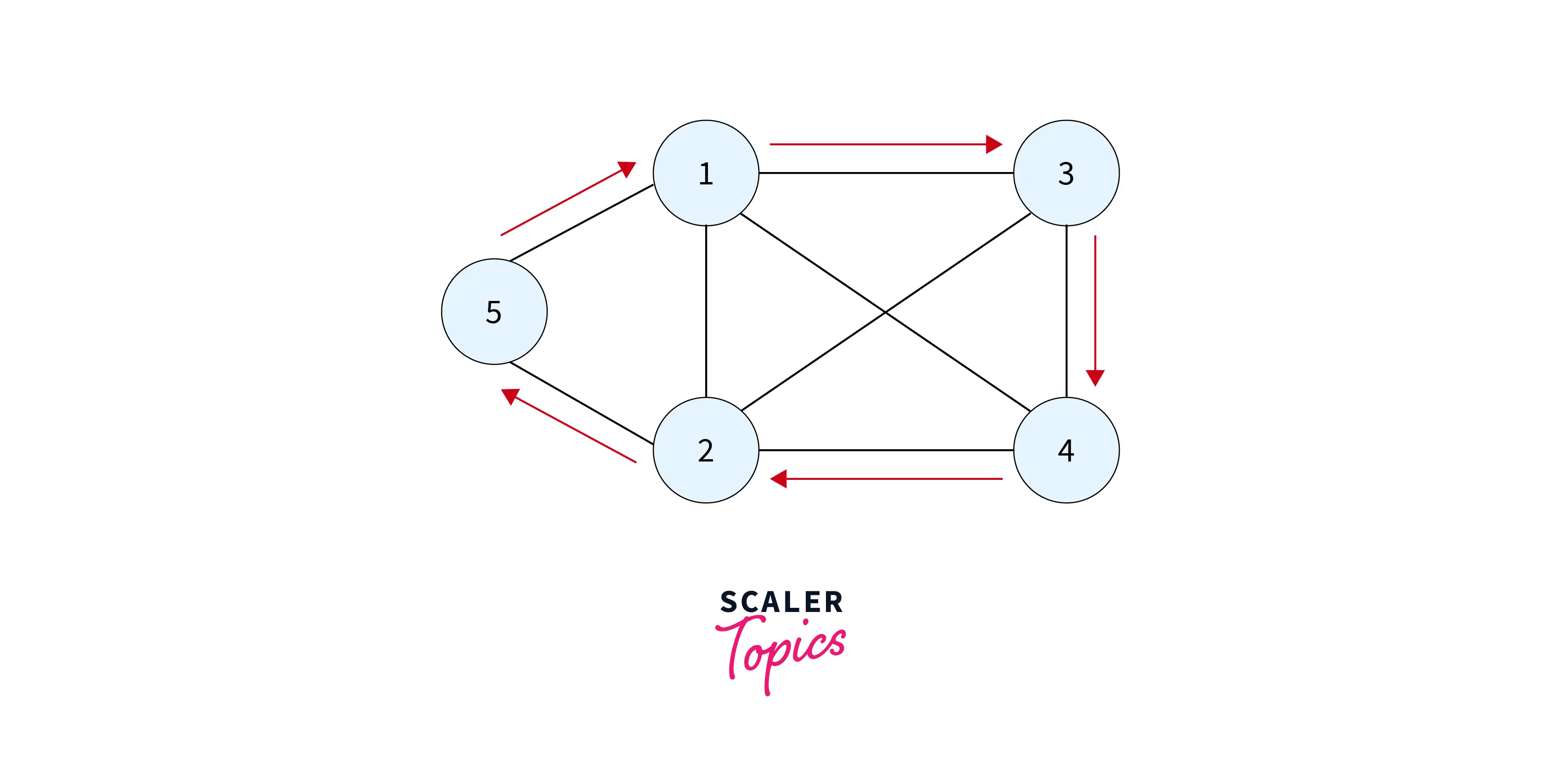
This is also a Hamiltonian circuit. Let's apply the Dirac's theorem on this graph i.e. $degree(v) >= N/2$ for all vertices: Here $N/2$ is 2 and let's see the degrees

Let's apply Ore's theorem on it i.e. $degree(u) + degree(v) >= N$ for any two non-adjacent vertices u and v.

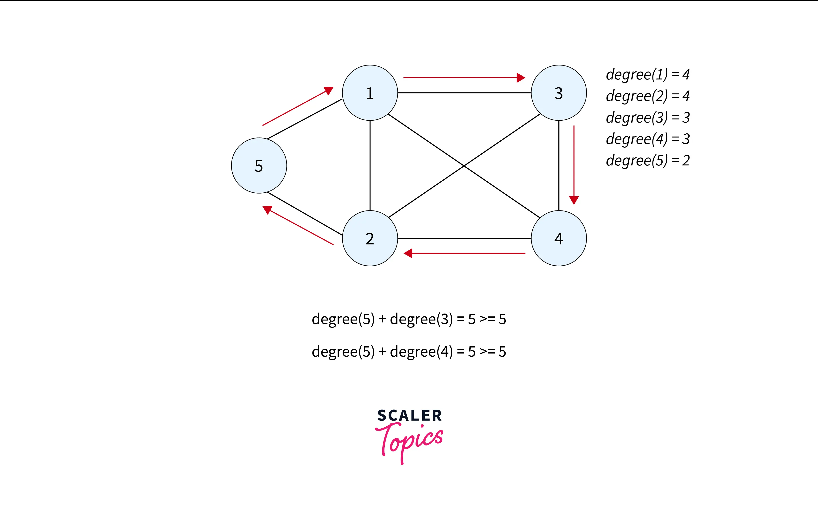
This is a Hamiltonian graph.