Joining Excel Sheets

Introduction

As data analysis becomes increasingly important in today's business world, the ability to combine data from multiple sources and perform complex calculations on it is a valuable skill. One of the most common scenarios where this is necessary is when working with Excel spreadsheets. Often, data that needs to be analyzed is spread across multiple worksheets or workbooks. In such cases, joining Excel sheets is a necessary step to get a comprehensive view of the data and perform useful analysis.

Joining Excel sheets involves combining data from two or more worksheets into a single sheet. This can be done in several ways, including using Excel's built-in functionality, such as the VLOOKUP function or Power Query. Joining Excel sheets can help you identify patterns and trends that may be hidden when looking at individual worksheets in isolation.

Joining Excel sheets is particularly useful when working with large data sets that are too large to fit into a single worksheet. By splitting the data into multiple sheets and joining them later, you can perform complex analyses while keeping the data organized and easy to manage. Joining Excel sheets can also help you identify inconsistencies in the data, such as missing or duplicate values, which can affect the accuracy of your analysis.

Overall, mastering the art of joining Excel sheets is an essential skill for any data analyst or business professional who works with data. By combining data from multiple sources and performing useful analysis on it, you can gain valuable insights into your data and make more informed decisions.

Joining Excel Sheets

Joining Excel sheets, also known as merging or consolidating, is the process of combining data from multiple sheets into a single sheet in Microsoft Excel. This can be helpful when you have data spread across multiple sheets and you want to analyze or summarize it in a single sheet. Excel provides several methods for joining sheets, including using built-in functions, data consolidation, and third-party add-ins. Here are some common ways to join Excel sheets:

• Copy and Paste:
  One of the simplest ways to join Excel sheets is to manually copy and paste the data from one sheet to another. To do this, select the data you want to copy in the source sheet, right-click and choose "Copy", then go to the destination sheet and right-click where you want to paste the data and choose "Paste". You can repeat this process for each sheet you want to join.
• Using the CONCATENATE Function:
  Excel's CONCATENATE function allows you to join data from different cells or sheets into a single cell. To use this function, enter the formula "=CONCATENATE()" in the destination cell where you want to join the data, then select the cells or sheets you want to combine, separated by commas, and close the parenthesis. For example, if you want to join data from cells A1 and B1 in Sheet1 and cells A1 and B1 in Sheet2, the formula would be "=CONCATENATE(Sheet1!A1, Sheet1!B1, Sheet2!A1, Sheet2!B1)".
• Using the VLOOKUP Function:
  The VLOOKUP function in Excel can also be used to join data from different sheets based on a common key. For example, if you have a column with unique identifiers in both the source and destination sheets, you can use VLOOKUP to match the identifiers and retrieve data from other columns in the source sheet. To use VLOOKUP, enter the formula "=VLOOKUP()" in the destination cell where you want to join the data, then specify the identifier you want to match, the range of cells in the source sheet where the data is located, and the column number or label of the data you want to retrieve.
• Using Data Consolidation:
  Excel's Data Consolidation feature allows you to combine data from multiple sheets into a single sheet automatically. To use this feature, go to the "Data" tab in Excel, click on "Consolidate" in the "Data Tools" group, and follow the prompts to select the sheets and ranges you want to consolidate. You can choose to consolidate data by position (e.g., same cell addresses across sheets) or by category (e.g., data with the same labels across sheets).

How to Merge Two Excel Spreadsheets?

Merging two Excel spreadsheets can be done using different methods, including combining by position or by category. Here's how you can merge two Excel spreadsheets using these methods:

Combine by Position

This method involves combining data from two Excel spreadsheets based on the position of the data, which means the data in the same cell addresses across both spreadsheets will be merged.

• Step 1:
  Open both Excel spreadsheets that you want to merge.
• Step 2:
  In the destination spreadsheet, go to the sheet where you want to combine the data.
• Step 3:
  Select the data range in the source spreadsheet that you want to merge.
• Step 4:
  Copy the selected data range in the source spreadsheet (Ctrl+C).
• Step 5:
  Go to the destination spreadsheet and paste the copied data range in the desired cell (Ctrl+V).
• Step 6:
  Repeat steps 3-5 for each data range you want to merge from the source spreadsheet.

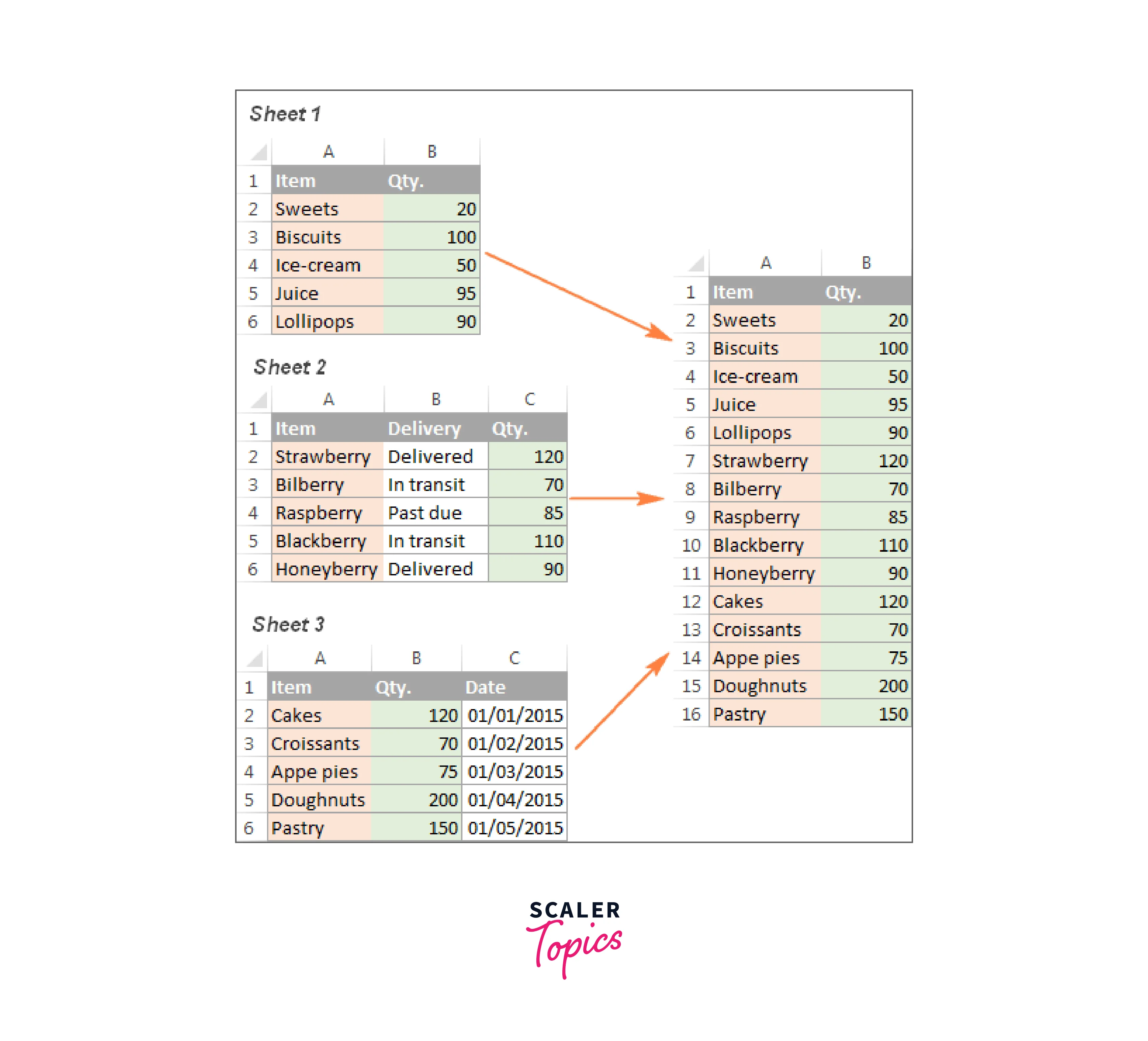
Combine by Category

This method involves combining data from two Excel spreadsheets based on categories or labels, which means data with the same labels across both spreadsheets will be merged.

• Step 1:
  Open both Excel spreadsheets that you want to merge.
• Step 2:
  In the destination spreadsheet, go to the sheet where you want to combine the data.
• Step 3:
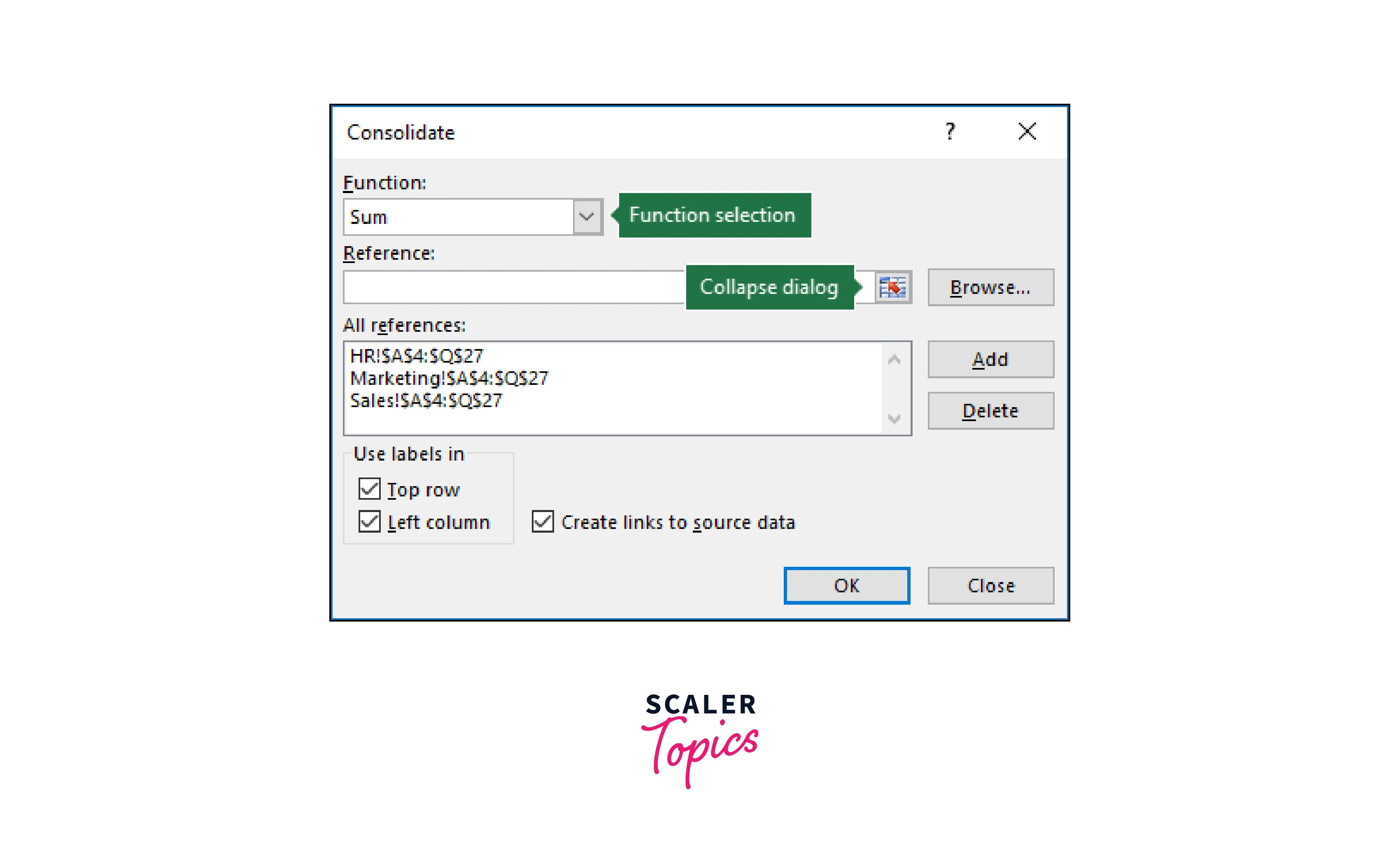
  Go to the "Data" tab in Excel and click on "Consolidate" in the "Data Tools" group.
• Step 4:
  In the "Consolidate" dialog box, select "Consolidate by Category" and click "Add" to specify the ranges in the source spreadsheet that you want to merge.
• Step 5:
  In the "Add References" dialog box, go to the source spreadsheet, select the data range you want to merge, and click "Add". Repeat this step for each data range you want to merge from the source spreadsheet.
• Step 6:
  Choose the consolidation method (e.g., sum, average, etc.) for merging the data and click "OK".
• Step 7:
  Choose the location in the destination spreadsheet where you want to place the merged data and click "OK".

Joining Data Types

Joining data types in Excel is a process of combining or merging two or more cells or columns that contain different types of data, such as text, numbers, dates, or other data formats, into a single cell or column. Excel provides various functions and methods to join or concatenate data types, allowing you to customize and combine data in a way that suits your needs. Here's how you can join different data types in Excel:

Using the CONCATENATE Function:

The CONCATENATE function in Excel allows you to join data from multiple cells or columns into a single cell or column. It is especially useful for combining text and numbers or text and dates.

Syntax:

• Step 1:
  In an empty cell where you want to join the data, enter the CONCATENATE function.
• Step 2:
  Specify the cells or text that you want to join within the parentheses. You can use text strings enclosed in double quotation marks, or cell references.
• Step 3:
  Separate multiple text or cell references with commas.
• Step 4:
  Close the parentheses and press Enter.

Example:

This formula joins the value in cell A2 with the text " - " and the value in cell B2, separated by a hyphen, into a single cell.

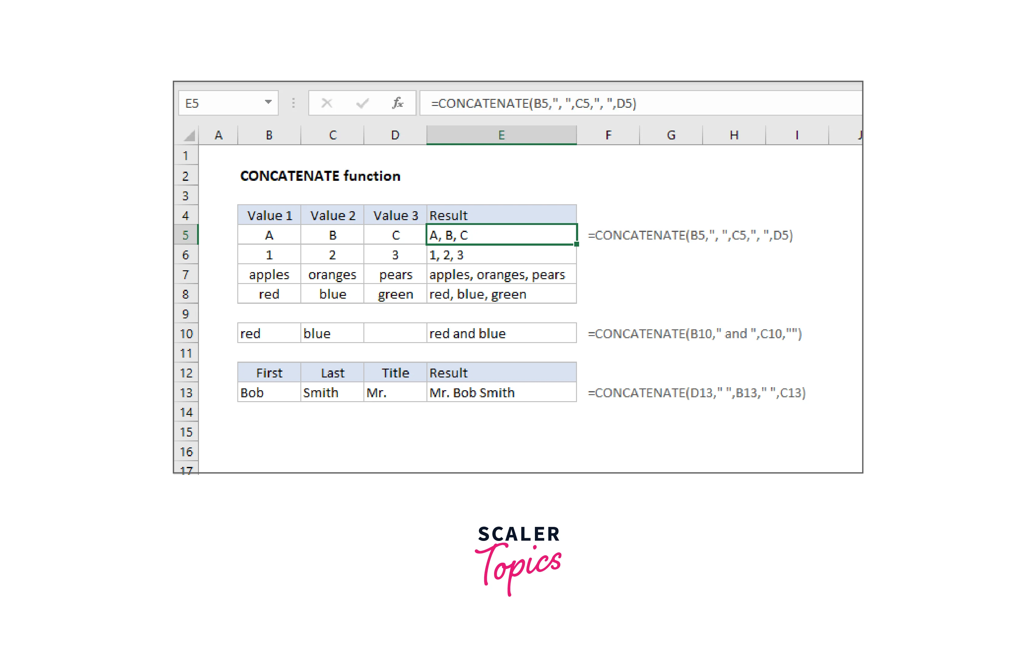
Using the "&" Operator:

In addition to the CONCATENATE function, you can also use the "&" operator in Excel to join data types. The "&" operator works similarly to the CONCATENATE function but with a shorter syntax. Syntax:

• Step 1:
  In an empty cell where you want to join the data, start with the first text or cell reference.
• Step 2:
  Type "&" followed by the next text or cell reference that you want to join.
• Step 3:
  Continue using "&" and additional text or cell references to concatenate the data.
• Step 4:
  Press Enter.

Example:

This formula joins the value in cell A2 with the text " - " and the value in cell B2, separated by a hyphen, into a single cell.

Using Text Functions:

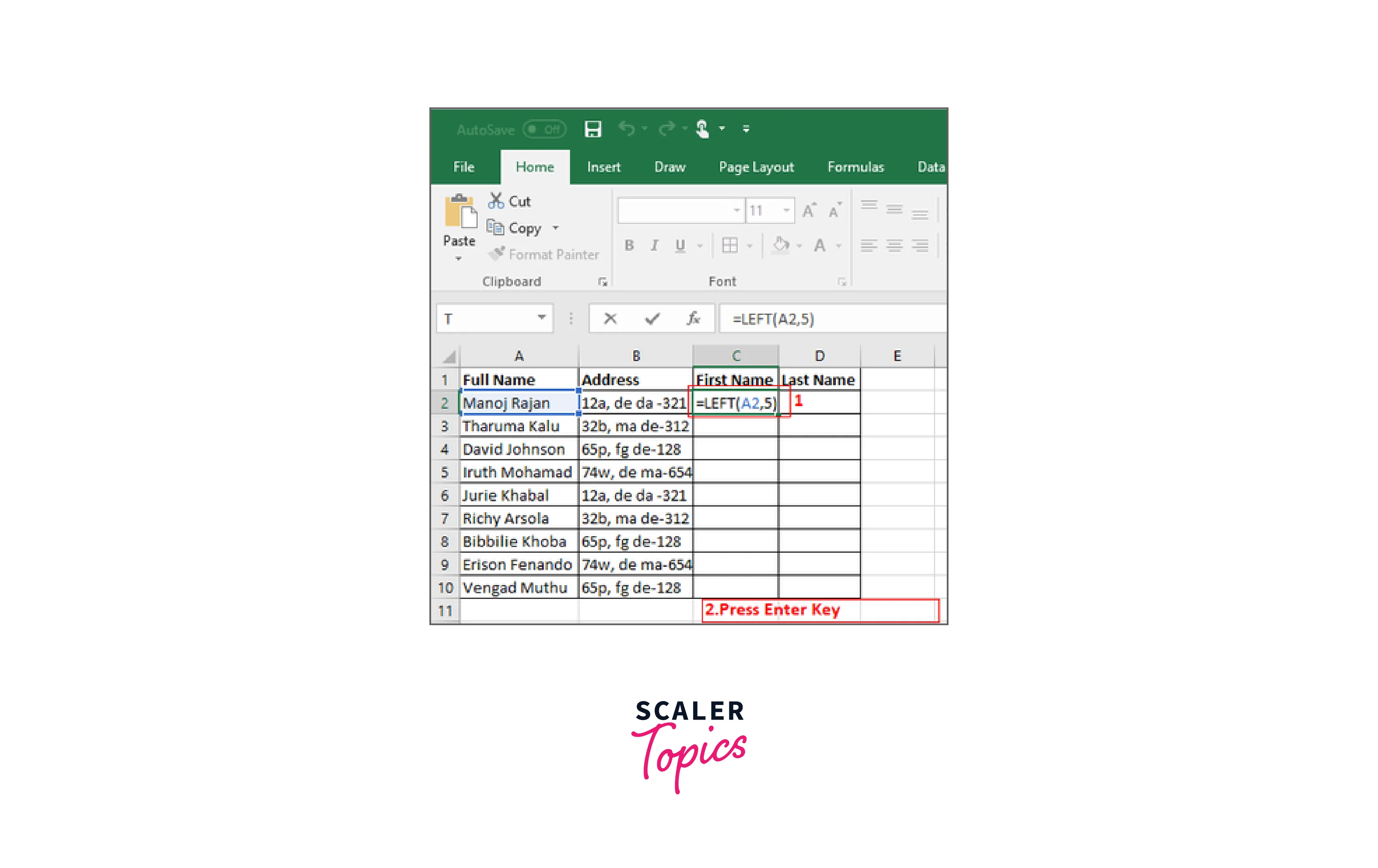
Excel provides several text functions, such as LEFT, RIGHT, MID, and SUBSTITUTE, that you can use in combination to join or manipulate data types. For example, you can use the LEFT function to extract a specific number of characters from the left of a text string and then join it with other text or data. Similarly, you can use the RIGHT function to extract characters from the right of a text string, the MID function to extract characters from the middle of a text string, and the SUBSTITUTE function to replace specific text within a string.

These text functions can be combined in various ways to customize and join data types in Excel, depending on your specific requirements.

Different Techniques for Joining Excel Sheets

Using VBA

VBA (Visual Basic for Applications) is a powerful tool that can be used in Microsoft Excel to automate tasks and manipulate data. When it comes to joining Excel sheets, VBA provides several techniques that can be used to achieve this.

• Copy and Paste:
  One of the simplest ways to join Excel sheets using VBA is by copying and pasting data from one sheet to another. This can be done using the Copy and Paste methods available in VBA. For example, you can loop through the cells in one sheet, copy the data, and then paste it into another sheet at the desired location.
• Consolidate Function:
  VBA allows you to use the built-in Consolidate function in Excel, which can be used to combine data from multiple sheets into one. You can specify the source ranges and the destination range using VBA code, and then use the Consolidate function to merge the data accordingly.
• Query Tables:
  VBA allows you to create and manipulate Query Tables, which are connections to external data sources such as other Excel sheets. You can use VBA code to create Query Tables and specify the data sources, and then use the Refresh method to update the data in the tables, effectively joining the data from different sheets.

INDEX

INDEX is a powerful function in Microsoft Excel that can be used to join or combine data from different sheets. It is a versatile function that can be used in various ways to consolidate data from multiple sheets into a single sheet. Here are some techniques for using INDEX to join Excel sheets:

• Vertical Joining: You can use INDEX to vertically join data from different sheets. For example, if you have data in Sheet1 in column A and data in Sheet2 in column B, you can use the formula "=INDEX(Sheet1!A: A, ROW())" in cell B1 of Sheet2 to pull data from Sheet1 into Sheet2. By dragging this formula down, you can pull data from multiple rows in Sheet1 and join it vertically with data in Sheet2.
• Horizontal Joining: You can also use INDEX to horizontally join data from different sheets. For example, if you have data in Sheet1 in row 1 and data in Sheet2 in row 2, you can use the formula "=INDEX(Sheet1!1:1, COLUMN())" in cell A2 of Sheet2 to pull data from Sheet1 into Sheet2. By dragging this formula across, you can pull data from multiple columns in Sheet1 and join it horizontally with data in Sheet2.

INDEX MATCH

INDEX MATCH is a powerful and flexible technique used in Microsoft Excel for joining data from different sheets. It is commonly used when you need to search for a value in one sheet (the "lookup value") and retrieve corresponding data from another sheet (the "match value") based on specific criteria.

The INDEX function is used to retrieve the value from a specified range in a sheet based on its row and column numbers. It has the following syntax: =INDEX(range, row_num, col_num), where "range" is the range of cells you want to search, "row_num" is the row number of the value you want to retrieve, and "col_num" is the column number of the value you want to retrieve.

The MATCH function is used to search for a specific value in a range of cells and return its relative position. It has the following syntax: =MATCH(lookup_value, lookup_range, match_type), where "lookup_value" is the value you want to search for, "lookup_range" is the range of cells you want to search in, and "match_type" specifies the type of match you want to perform (e.g., exact match or approximate match).

Power Query

Power Query is a powerful data transformation and data integration tool available in Microsoft Excel. It provides various techniques for joining Excel sheets, allowing users to merge and combine data from different worksheets or workbooks. Here are some different techniques for joining Excel sheets using Power Query:

• Append Queries:
  This technique allows you to vertically stack data from multiple worksheets or workbooks. You can append queries by going to the Power Query tab in Excel and selecting "Append Queries". You can then choose the worksheets or workbooks you want to combine and specify how you want the data to be appended, such as by stacking rows or columns. This is useful when you have similar data in different sheets that you want to combine into a single table.
• Merge Queries:
  This technique allows you to horizontally combine data from different worksheets or workbooks based on matching columns. You can merge queries by selecting "Merge Queries" from the Power Query tab in Excel. You can then choose the worksheets or workbooks you want to merge and specify the columns that you want to use as the key to join the data. You can choose different types of joins, such as inner join, left join, right join, or outer join, depending on how you want to combine the data.

What is VLOOKUP?

VLOOKUP stands for Vertical Lookup, and it is a built-in function in Excel that allows you to search for a value in the first column of a data range and retrieve a corresponding value from a specified column in the same row. VLOOKUP is commonly used for data analysis and reporting tasks, where you need to quickly retrieve data from a large data set based on specific criteria.

The syntax of the VLOOKUP function is as follows:

• lookup_value:
  The value you want to search for in the first column of the data range.
• table_array:
  The range of cells that contains the data you want to search in, including both the lookup column and the columns from which you want to retrieve data.
• col_index_num:
  The relative position of the column from which you want to retrieve data, where 1 corresponds to the first column in the data range, 2 corresponds to the second column, and so on.
• range_lookup:
  An optional parameter that specifies whether you want to perform an exact match (FALSE or 0) or an approximate match (TRUE or 1). If omitted, Excel assumes TRUE by default.

What is HLOOKUP?

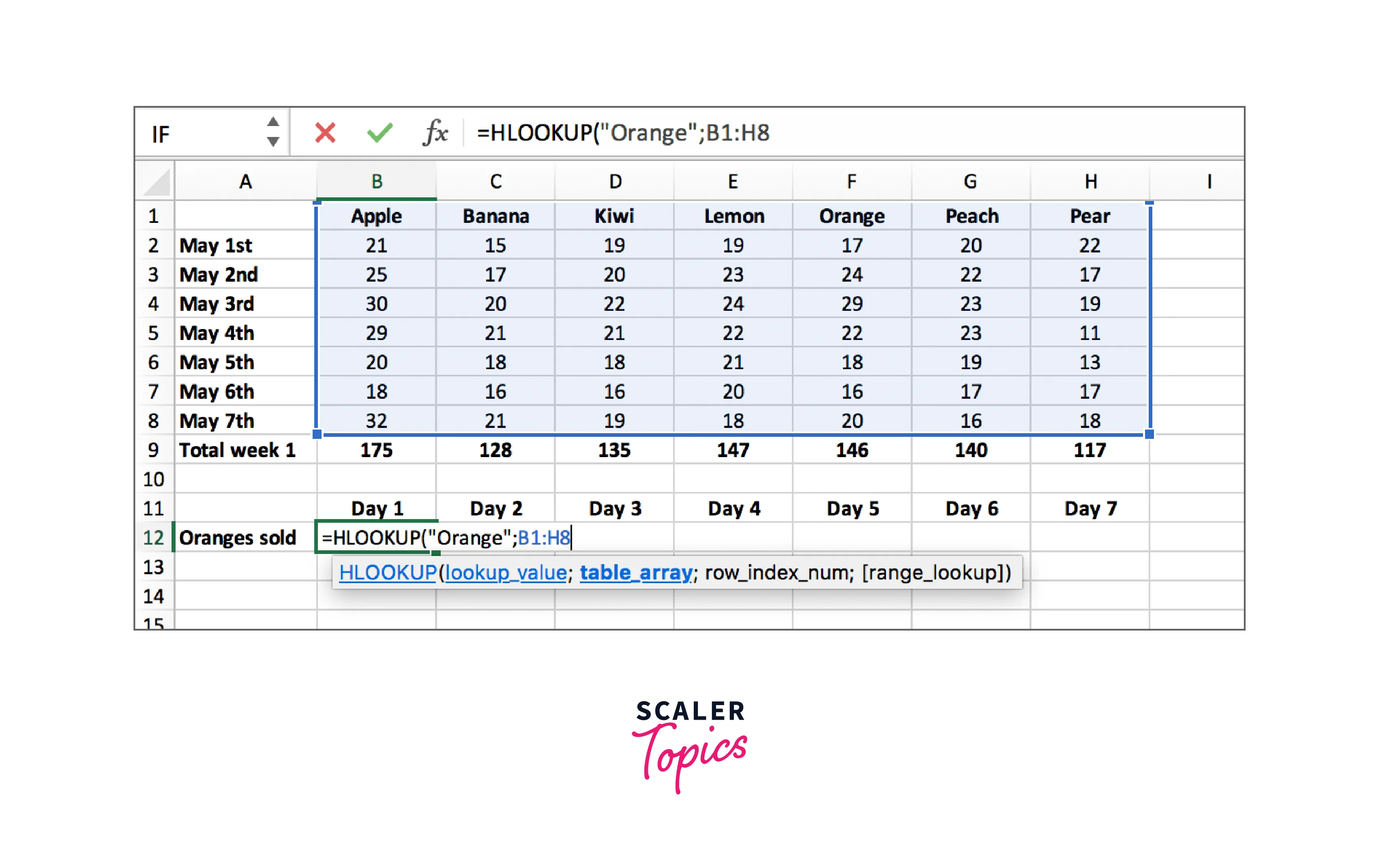
HLOOKUP, short for "Horizontal Lookup", is a function commonly used in spreadsheet software, such as Microsoft Excel or Google Sheets, to search for a value in the top row of a range and return a corresponding value from a row below that value. It is a type of lookup or search function that operates horizontally across rows, as opposed to VLOOKUP, which operates vertically down columns.

The syntax for HLOOKUP typically includes the following arguments:

• Lookup_value:
  The value you are searching for in the top row of the range.
• Table_array:
  The range of cells that contains the data you want to search through.
• Row_index_num:
  The row number within the table_array from which you want to retrieve a value.
• Range_lookup:
  An optional argument that specifies whether you want an exact match (FALSE) or an approximate match (TRUE) for the lookup_value. If omitted, it defaults to TRUE.

HLOOKUP is often used in spreadsheet applications for tasks such as retrieving data from a data table, looking up prices, or finding corresponding values for codes or identifiers. It is a powerful tool for searching and retrieving data horizontally, based on a specified value.

What is XLOOKUP?

XLOOKUP is a function in Microsoft Excel, which is a popular spreadsheet program, used for looking up and retrieving data from a specified range based on a given search criteria.

The XLOOKUP function allows you to search for a value in one column or row of a table, and then return a corresponding value from another column or row in the same table. It is particularly useful when dealing with large data sets or when you need to search for values in multiple columns or rows simultaneously.

The syntax for XLOOKUP is as follows:

where:

• lookup_value:
  The value you want to search for.
• lookup_array:
  The range of cells that contains the value you want to search in.
• return_array:
  The range of cells from which you want to return a corresponding value.
• if_not_found:
  (optional) The value to return if the lookup_value is not found in the lookup_array. If not specified, Excel will return an error.
• match_mode:
  (optional) Specifies how the lookup_value should be matched in the lookup_array. It can be set to exact match (0), approximate match (1), or wildcard match (2). The default is 1 (approximate match).
• search_mode:
  (optional) Specifies whether to search in rows (1), columns (2), or both (3) in the lookup_array. The default is 1 (rows).
• XLOOKUP is a powerful tool for advanced data lookup and retrieval in Excel, and it offers more flexibility and functionality compared to older lookup functions such as VLOOKUP and HLOOKUP. It is widely used in various industries and professions for tasks such as data analysis, reporting, and financial modeling.

Tips For Merging Two Spreadsheets in Excel

• Make sure the data in both spreadsheets is clean and organized:
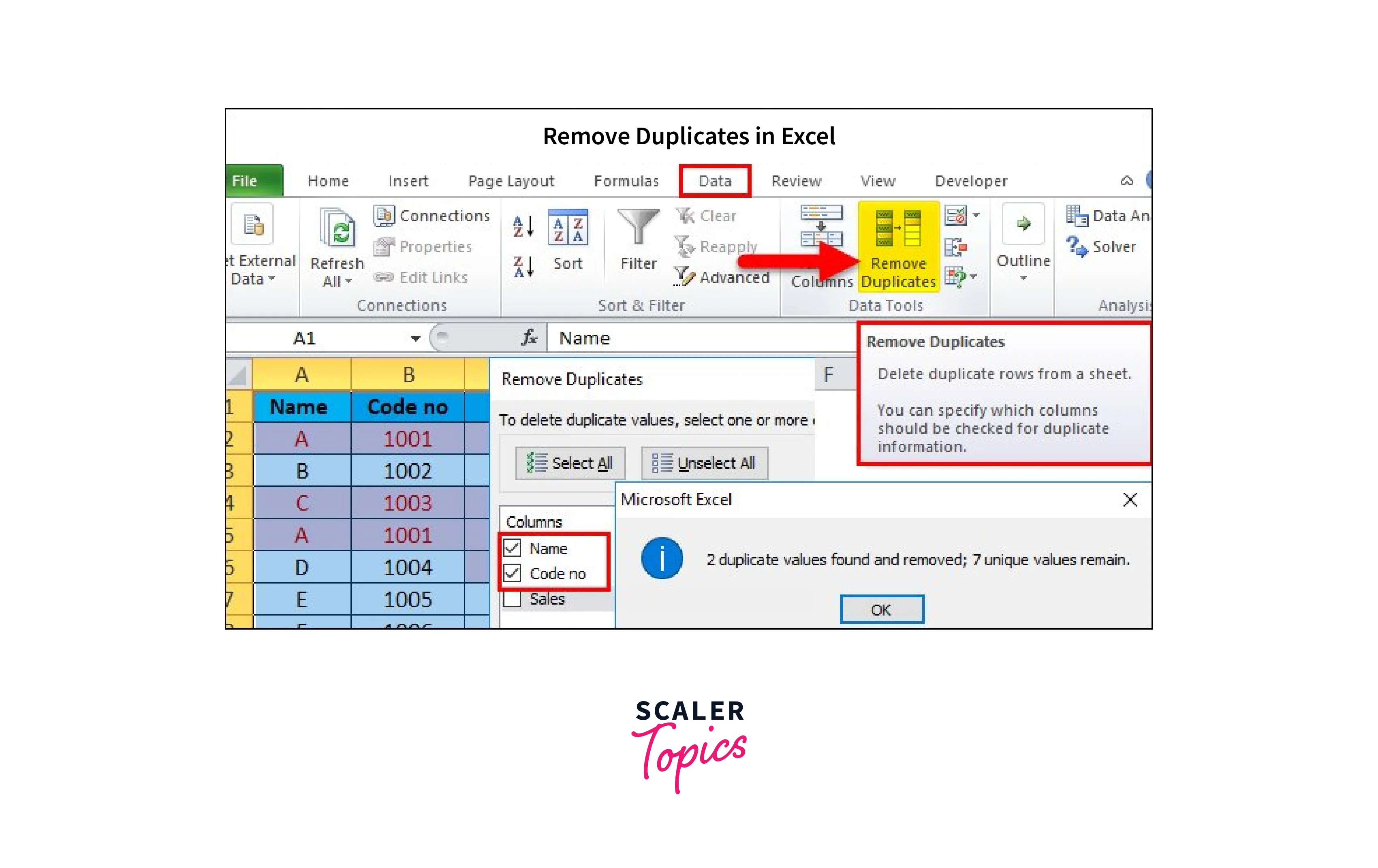
  Before merging two spreadsheets, it's important to ensure that the data in both sheets are clean and organized. This includes removing any duplicate rows, correcting any errors or inconsistencies in data, and ensuring that the data is formatted consistently.
• Identify a common column:
  To merge two spreadsheets, you need to identify a common column that exists in both sheets. This could be a unique identifier, such as an employee ID or a product code, which can be used as a key to match and merge the data in both sheets.
• Use Excel's built-in data merging tools:
  Excel provides several built-in data merging tools that can help you combine data from two or more sheets. These tools include the "Consolidate" feature, which allows you to combine data from multiple ranges or sheets into a single sheet, and the "Merge & Center" feature, which allows you to merge cells and center the content in the merged cells.
• Use formulas to combine data:
  You can also use formulas in Excel to merge data from two or more sheets. For example, you can use the VLOOKUP or INDEX-MATCH functions to look up and retrieve data from one sheet based on a common column in another sheet. You can also use concatenation or text manipulation functions to merge text or data from different cells into a single cell.