How to Extract Data from Excel?
Overview
Excel is a powerful tool for data analysis, and one of its key features is the ability to extract and manipulate data. There are several types of data extraction in Excel, including filtering, sorting, and using functions such as VLOOKUP and INDEX-MATCH. Filtering allows you to display only the needed data by selecting specific criteria. Sorting allows you to rearrange data based on specific columns in ascending or descending order. Finally, VLOOKUP and INDEX-MATCH allow you to search for data in one table and retrieve matching data from another. These data extraction techniques are essential for working with large data sets and can help you gain insights and make informed decisions. Learning how to extract data from Excel is crucial for effectively working with your datasets.
What is Data Extraction?
Data extraction is the process of retrieving specific information from a larger dataset. Excel is a commonly used tool for data management and analysis, and it provides several methods for extracting data from a workbook. These methods include formulas such as INDEX-MATCH, VLOOKUP, HLOOKUP, SUMIF, and tools like the Filter and Sort functions. In addition, scripting languages like Python and third-party software applications can extract data from Excel sheets. The specific method chosen depends on the needs and requirements of the data analysis task. It's crucial to understand how to extract data from Excel. Overall, Excel is a powerful platform for data extraction and management, providing a range of options for retrieving and manipulating data.
Types of Data Extraction
Data extraction is collecting data from various sources for transformation, storage, or feeding it to another system for subsequent analysis. Data extraction is divided into two categories: logical extraction and physical extraction.
Logical Extraction:
Methods of Logical Extraction:
- Full Extraction:
It is a method of extraction in which all data is extracted at once from the source without any filters or modifications, just like taking all the fruits from the original basket and putting them into the new basket without leaving anything behind. It maintains the relationships and integrity of the data. In this method, we don't need to keep track of data source changes.- Full Extraction is useful when moving data to a new system or backing up the source data.
- As a result, it takes more time and resources than any other extraction method.
- Incremental Extraction:
It is a method of extraction that involves extracting only the data that has been added/removed/updated since the last extraction rather than extracting all of the data every time.- As a result, it is less time-consuming and more efficient.
Physical Extraction:
Depending on the chosen logical extraction method and the source site's capabilities and limits, methods of physical extraction:
- Online Extraction:
The data or information is taken directly from the source system to the data warehouse. - Offline Extraction:
The data or information is not taken directly from the source system to the data warehouse and occurs outside the source system.
Understanding how to extract data from Excel is vital for working with datasets in various scenarios. By using Excel's built-in functions and features, you can efficiently extract the necessary information from your data, making your analysis more effective and accurate. By mastering data extraction techniques, you can gain insights and make informed decisions based on the information contained within your Excel workbooks. Becoming proficient in how to extract data from Excel will enable you to maximize the potential of your data analysis tasks.
Methods to Extract Data from an Excel Sheet
Using VLOOKUP Function
VLOOKUP is a built-in function in Excel that allows extracting data from a table or range based on a specific lookup value.
- VLOOKUP is referred to as a premade function as well.
- Premade Function in Excel: The AND function is known as a permade function, which returns TRUE or FALSE based on two or more conditions.
- It is typed = AND and takes two or more conditions.
Syntax: VLOOKUP Function
where,
- Lookup value:
The cell that has the unique identifier. - Table range:
The range of the table, including all cells. - Column number:
The number of the column that has the data you're looking for. - True/False:
This argument is optional. Determines whether to search for an exact match or an approximate match.- In Column number, the counting starts from the leftmost column in the table, which equals 1.
- True means an approximate match, while False means an exact match.
Range Name in Excel
Defining a range name makes it easier to reference the cells or groups of cells in formulas and functions. Easier to work and extract data even if the cells are located in different parts of the worksheet.
Steps in Defining - Range Names in Excel
- Go to the source data worksheet.
- Select all cells or a range of cells we want to name.
Hint: select all cells from A5 to end
- In Windows: click A5, then press Ctrl-Shift-End
- In Mac: click A5, then press Command-Shift-End
- In place of A5, written above the column 'A', change it to your range name.
- Range name is "scalar".
- Now use the word "scalar" in place of table range.
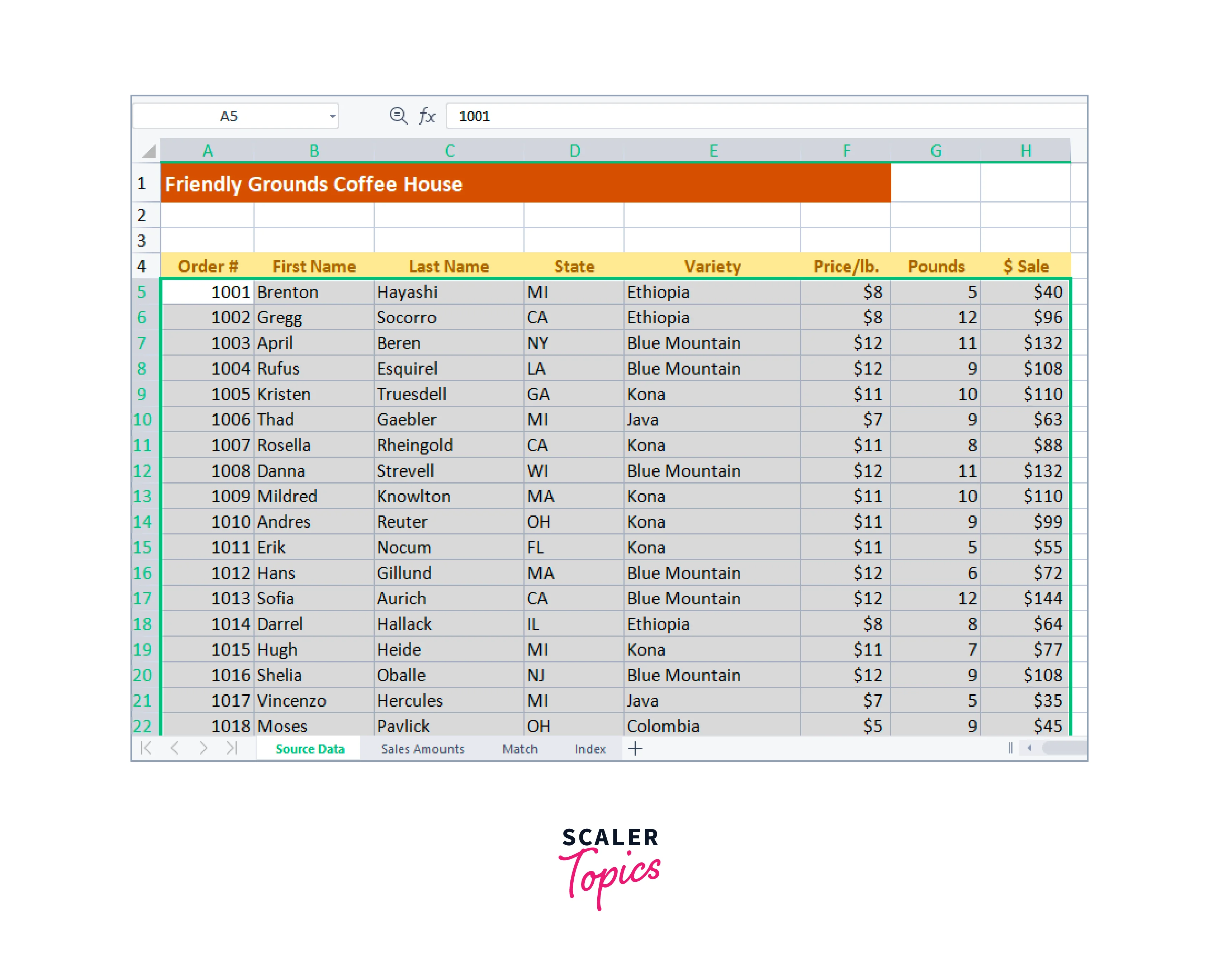
Extracting data using the formula
So, to extract the data from Excel using the VLOOKUP formula.
-
Step - 1:
Open the required worksheet.Here, open the "Sales Amount" worksheet.
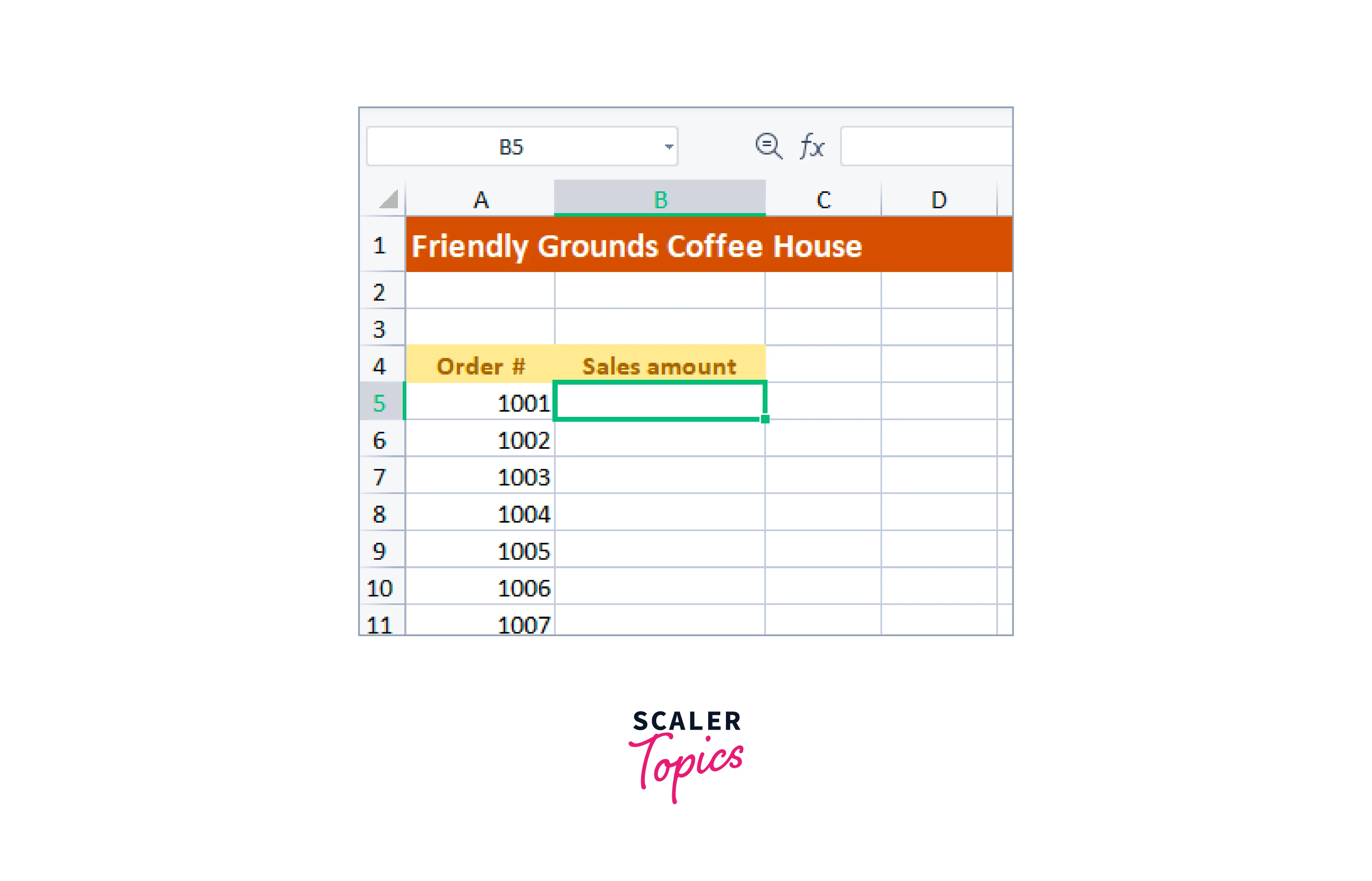
-
Step - 2:
Select the required cell for using the formula. -
Step - 3:
Enter the formula and press Enter.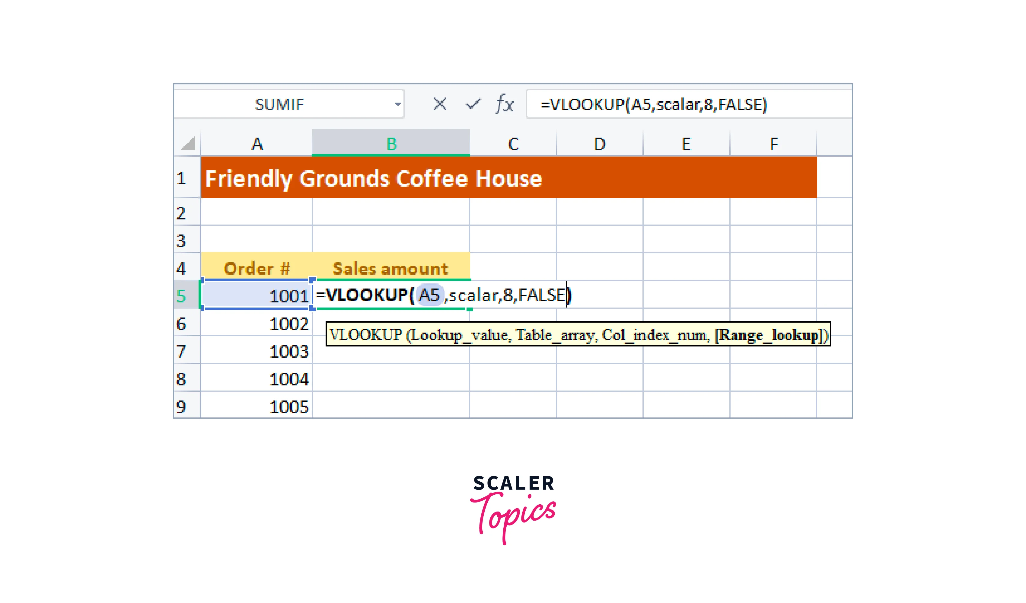
- Here, select cell B5.
- Type formula in B5: =VLOOKUP(A5,scalar,8,FALSE)
-
Step - 4:
Result will be shown in the cell.
Drag the mouse and double-click to fill the values down the column.
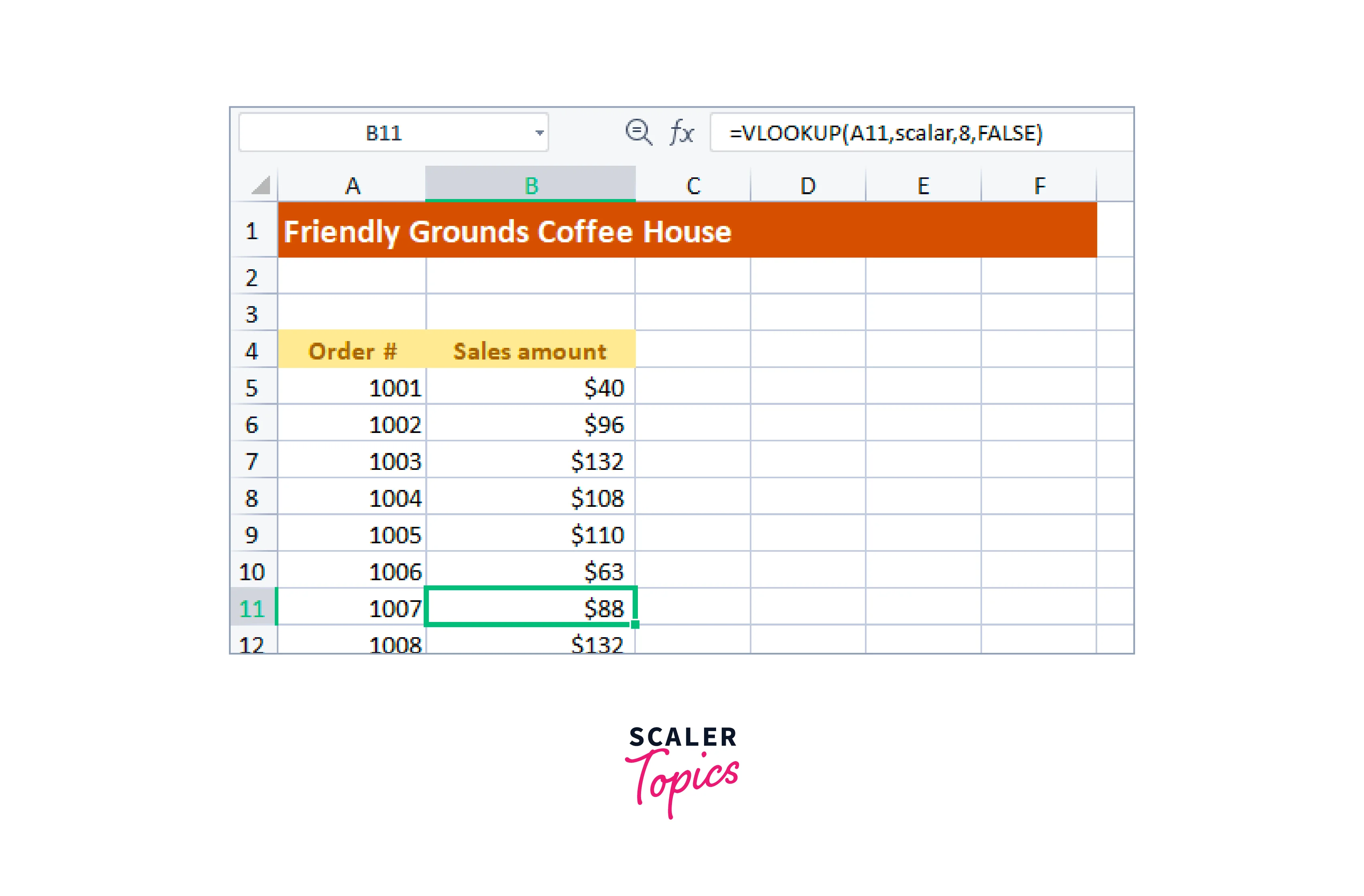
Note:
The VLOOKUP function has limitations and can sometimes be slow and inefficient for large datasets or complex queries.
Using with INDEX Function
The INDEX function is a tool for extracting data from various cells. It allows you to retrieve a specific value from a table or range of cells based on its position or location within the range without specifying the lookup column.
Syntax:
where,
- Range:
Takes the range of cells or tables from which you want to retrieve a value - Row Number:
The row number within the range from which you want to retrieve a value. - Column Number:
It is the column number within the range from which you want to retrieve a value. The column number is an optional field.
Extracting data from Excel using Index Function:
The INDEX function is similar to VLOOKUP.
To find what's contained in row 9, column 3 of the table.
-
Step - 1:
Open the worksheet.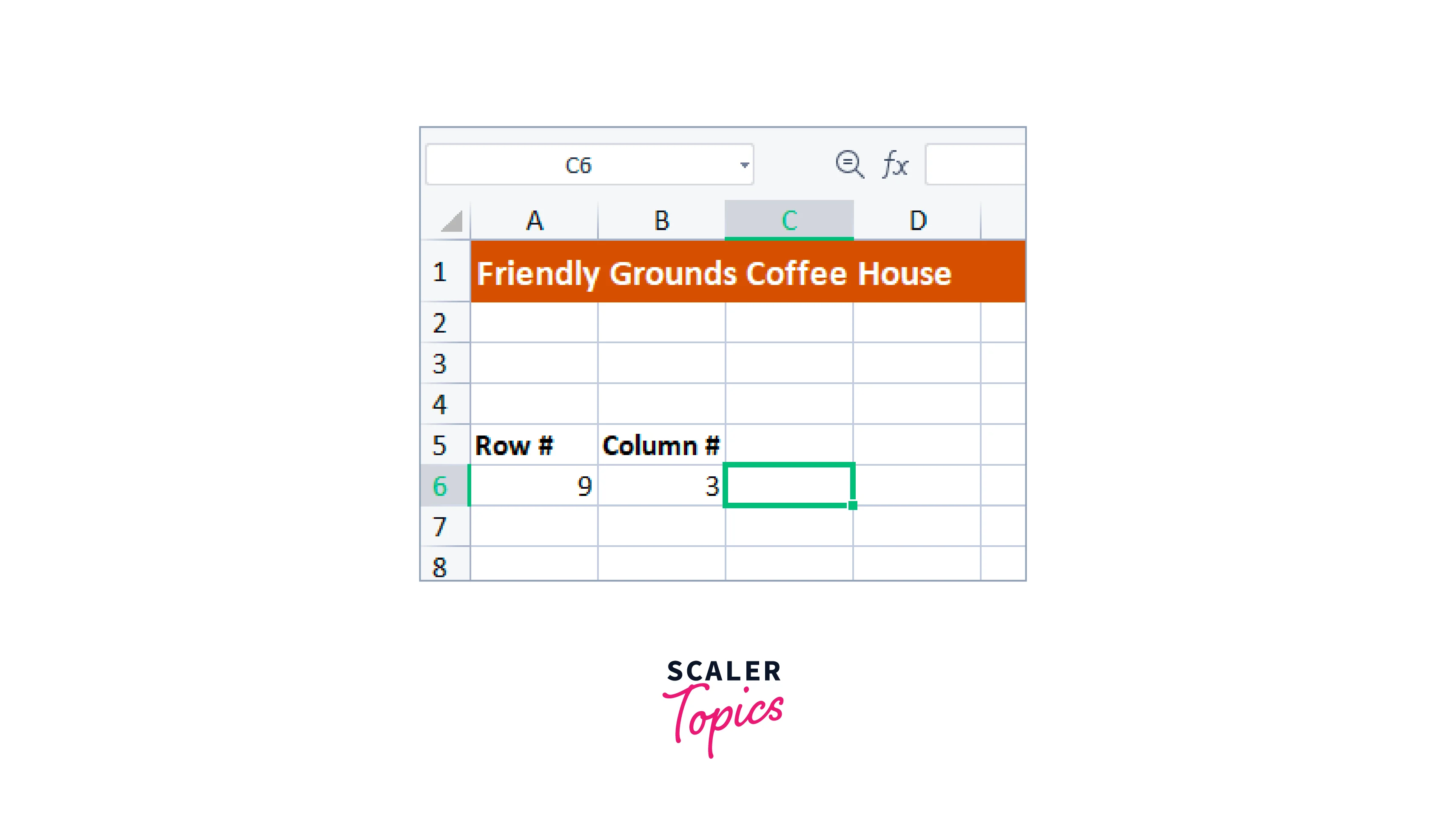
-
Step - 2:
In C6,enter the formula.
Here, we use the same range name, "scalar," as in the previous case.
-
Step - 3:
Check the result in C6.
Change the values of A6 and B6, and the result in C6 will show different results.
With the Help of Name Box
With the help of Name Box, you can automatically update the changes made in the source worksheet to the destination worksheet.
Here, the destination worksheet means the worksheet where the data has been copied or stored.
Suppose we have two worksheets.
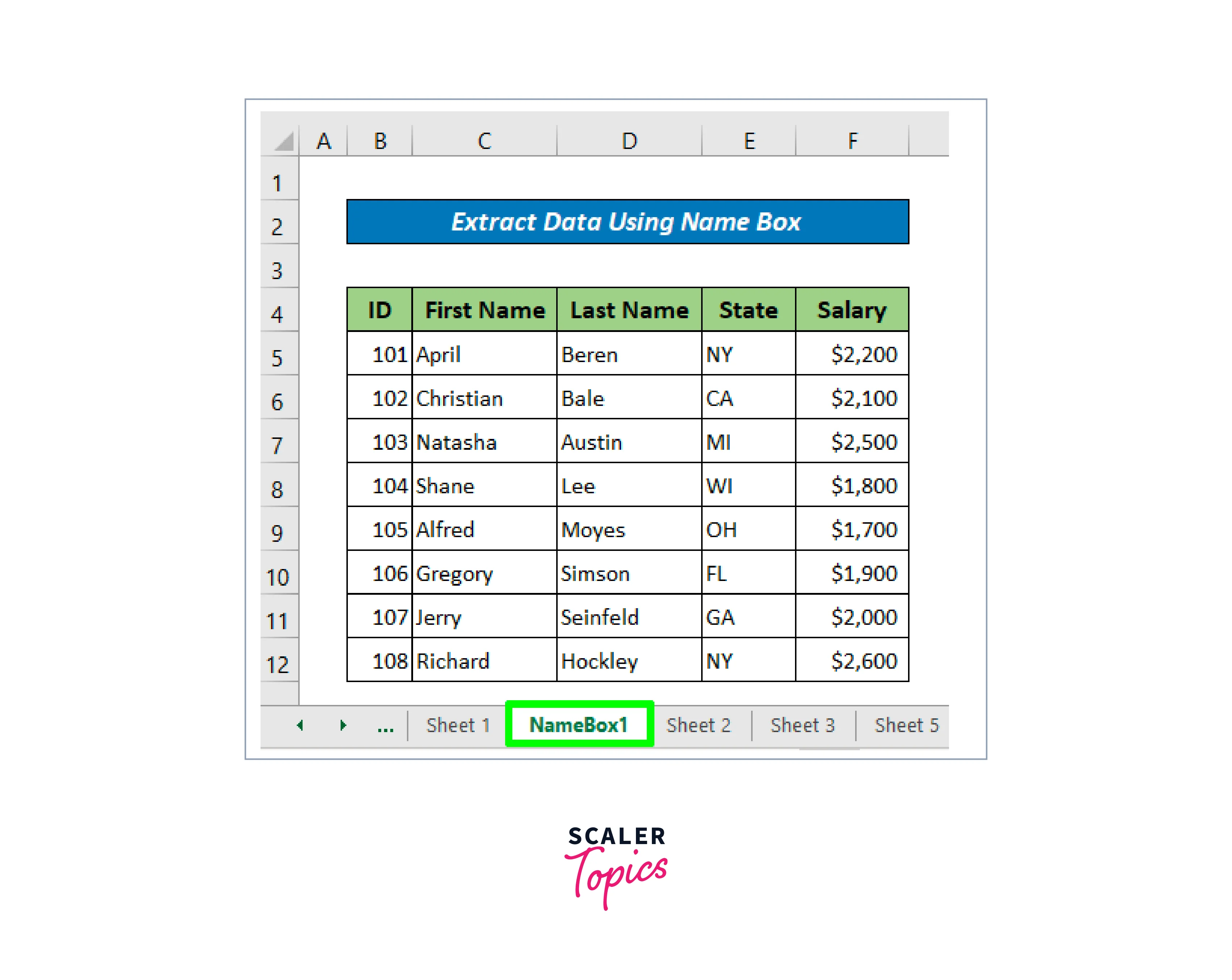
- Source worksheet: NameBox1
- Destination worksheet: NameBox2
-
Step - 1:
Select the destination cell. -
Step - 2:
Enter the formula, begin with "=". -
Step - 3:
After "=", type the name of the sheet where the data is located, followed by an exclamation point (!).For example, if the sheet is named "Sheet2", type "Sheet2!".
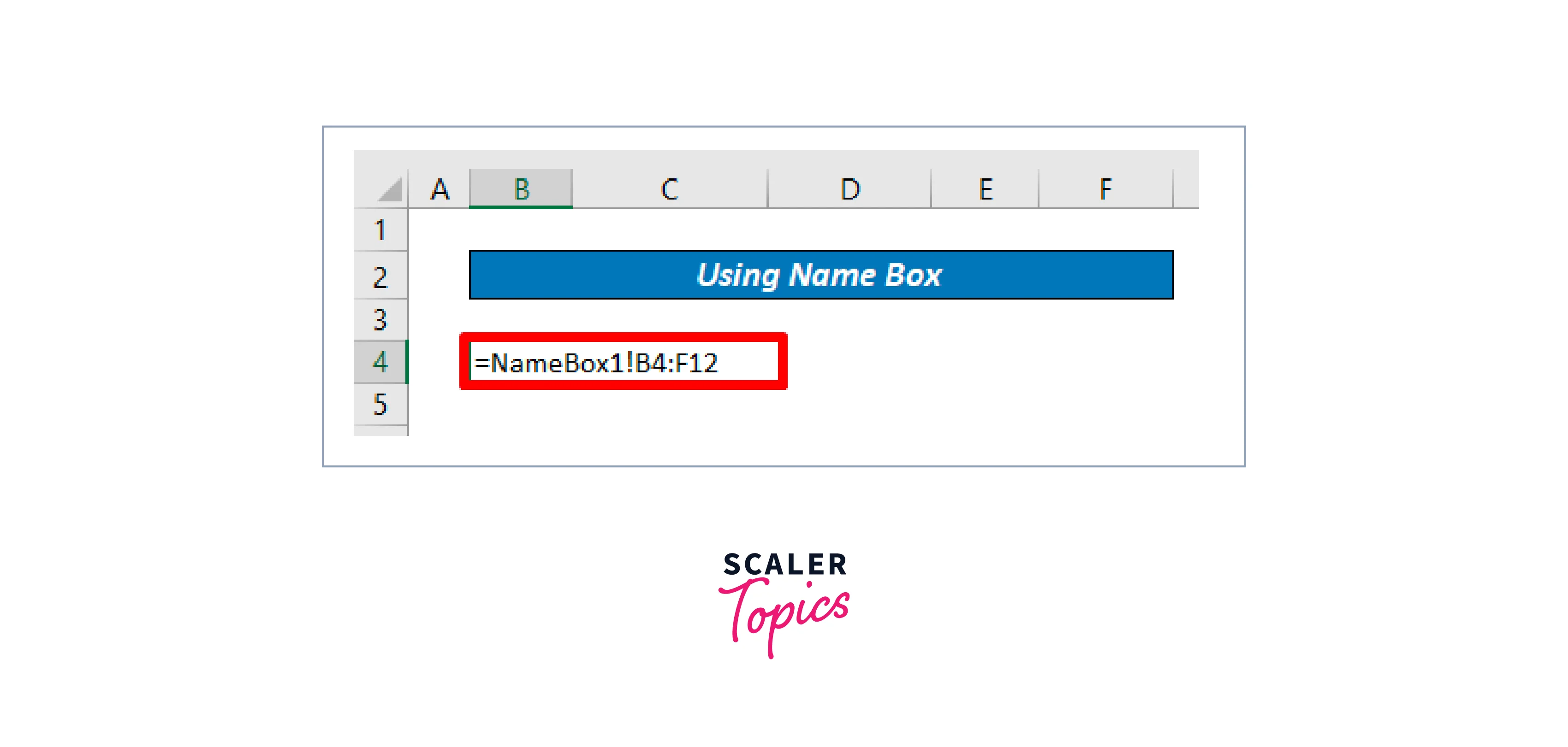
=NameBox1!B4:F12 means extract the data ranging from B4 to F12 from NameBox1 worksheet.
-
Step - 4:
Result will be shown in the destination worksheet.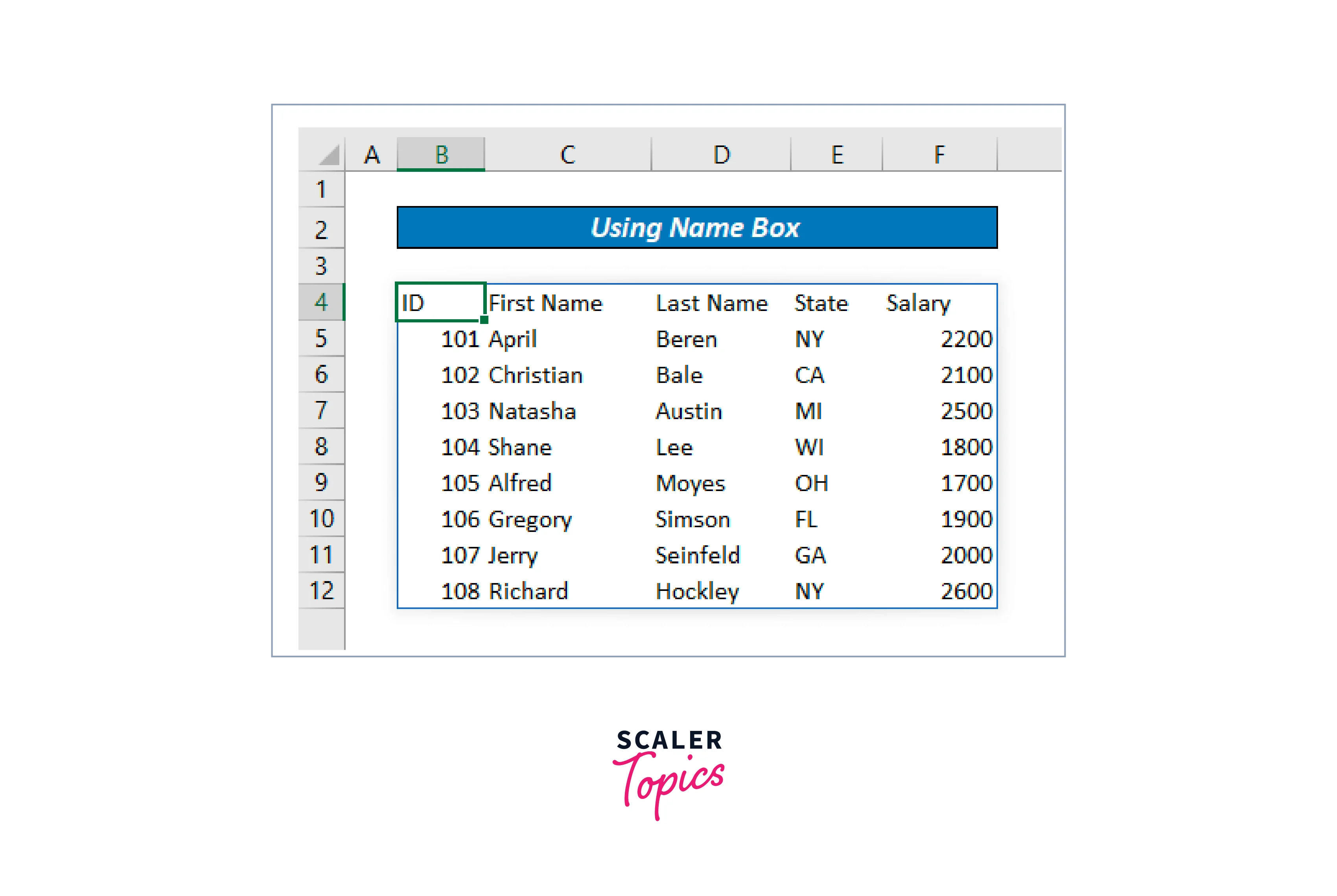 Data extracted and copied in the NameBox2.
Using INDEX-MATCH Formula
The INDEX-MATCH function is a combination of two functions: INDEX and MATCH.
- The INDEX function returns the value of a cell in a specified row and column of a table.
- The MATCH function returns the position of a specified value in a range of cells.
Syntax of Match Function
where,
- [match_type]: This optional field can have three values: -1, 0, or 1.
To extract the data from Excel of ID sheet 1 to sheet 3, using the dataset as using "With The Help Of Name Box".
-
Step - 1:
Select the destination cell. -
Step - 2:
Enter the formula and press Enter.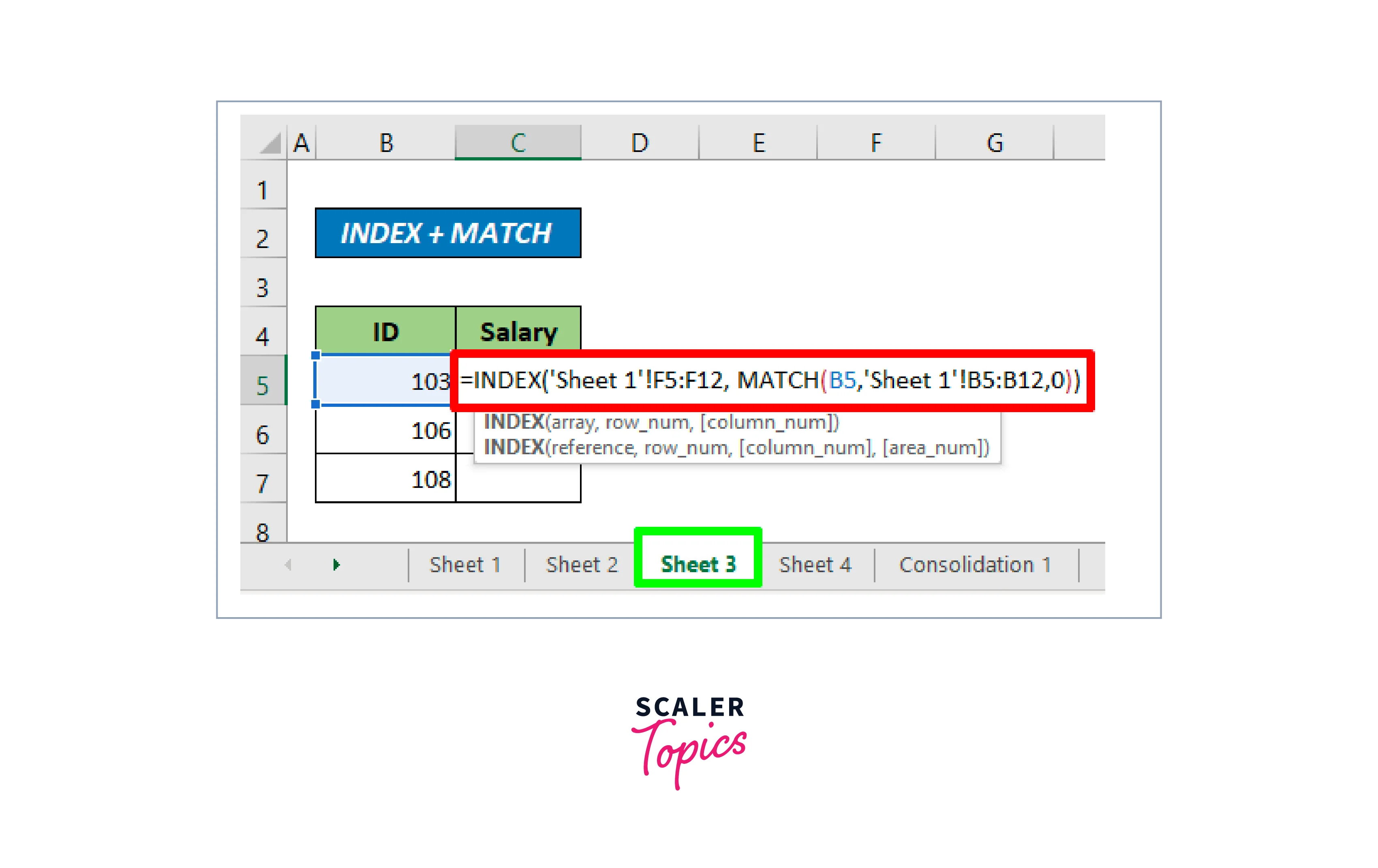
MATCH function
- B13 is the lookup_value.
- 'Sheet 1'!B5:B12 is the data range of cells to search for a specified value.
- The last argument is "0", indicating an exact match is required.
- It returns three because the value is in row number 3.
INDEX function
- It uses the result of the MATCH function as the row argument to return the value from the corresponding cell in the 'Sheet 1'!F5:F12 range of cells.
-
Step - 3:
Result will be shown.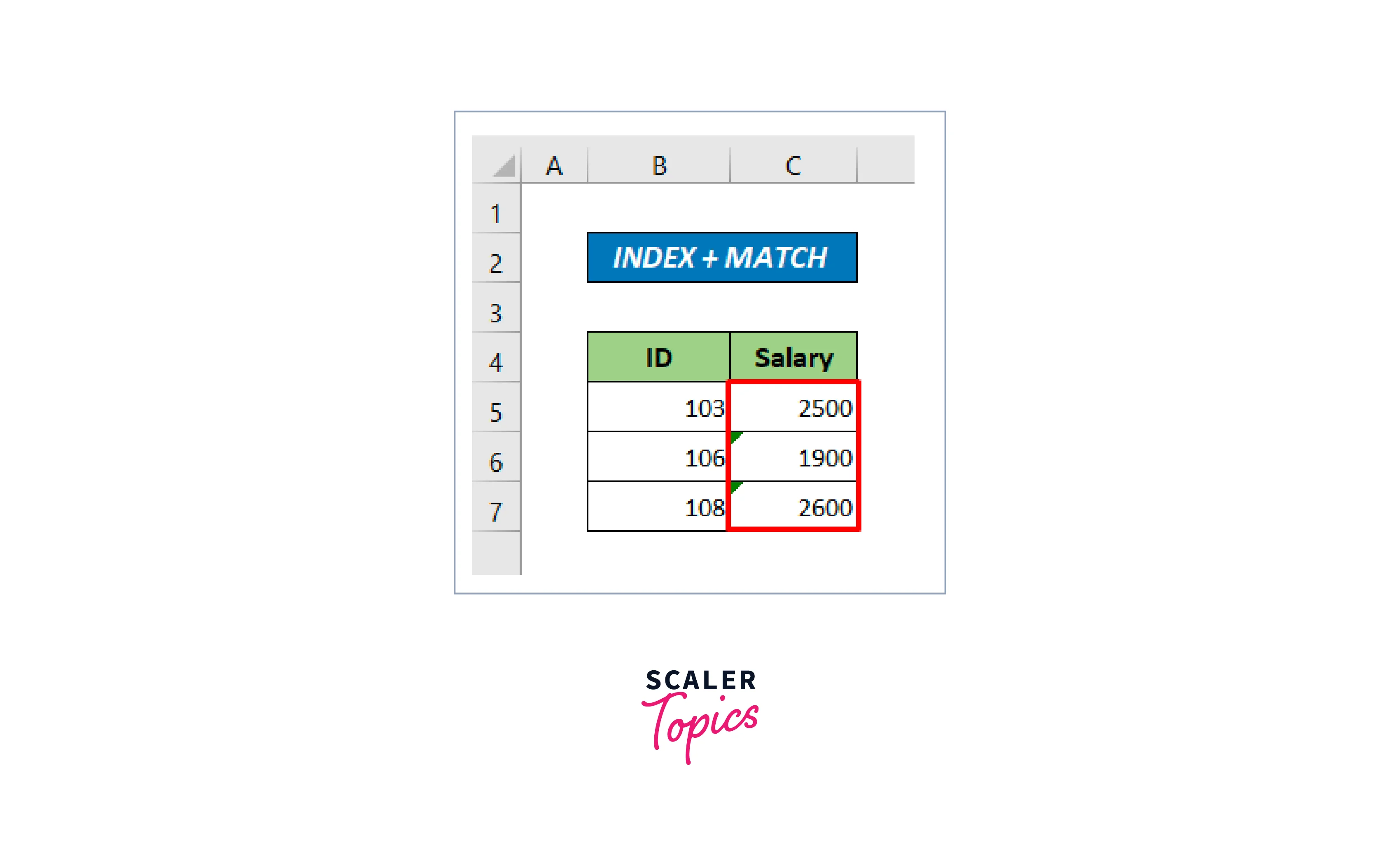
Here, this formula searches for cell B13 in the 'Sheet 1'!B5:B12 range of cells and returns the corresponding value from the 'Sheet 1'!F5:F12 range.
Using Data Consolidation Tool
Here, we will understand how to extract data from Excel using the data consolidation tool.
Given two datasets in the same Excel worksheet.
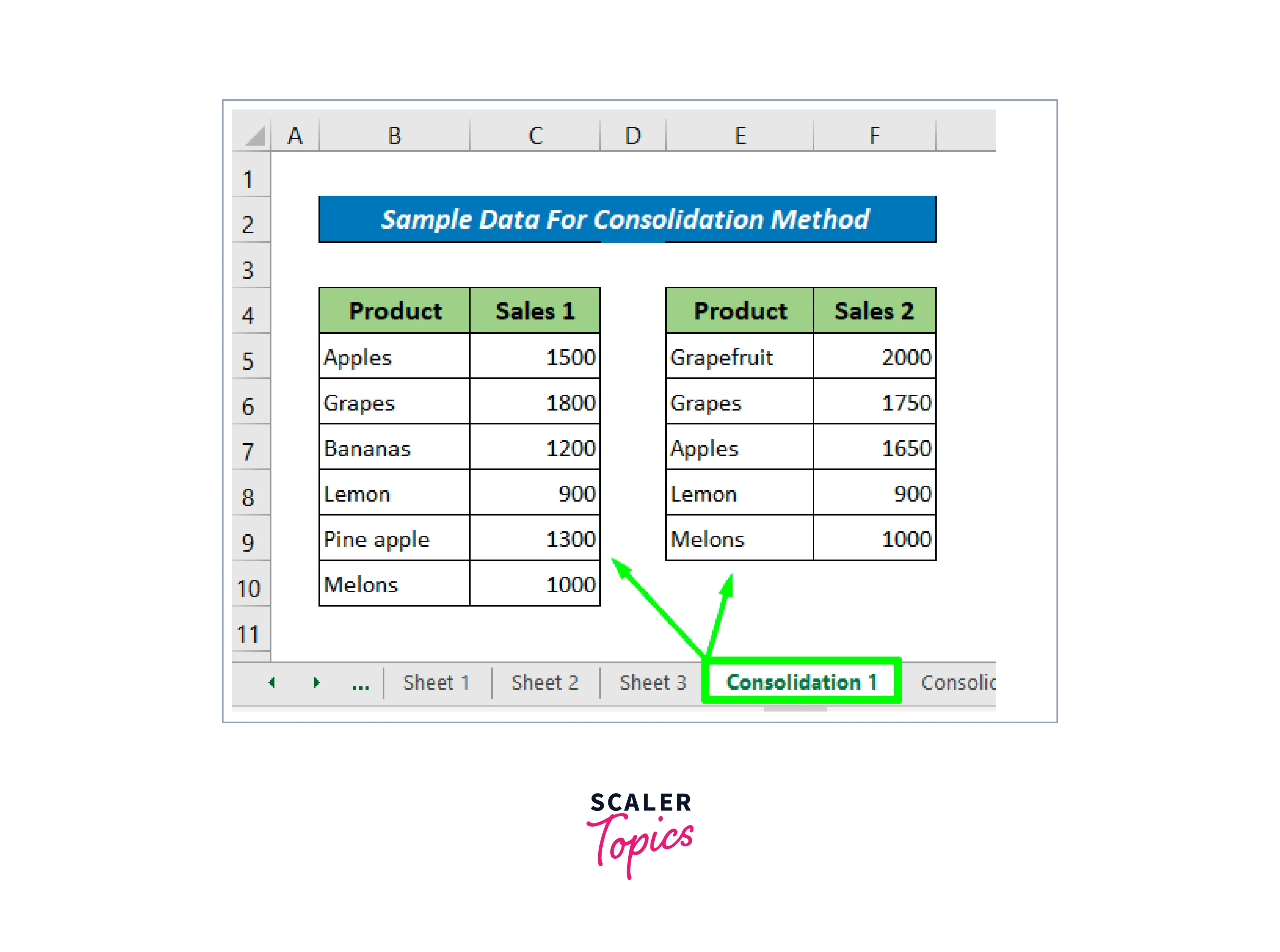
-
Step - 1:
Go to the destination sheet. Then, select a cell for the result. -
Step - 2:
Next is to open the Data tab >> the Data Tools group >> Click on the Consolidate icon opening a Consolidate dialog box.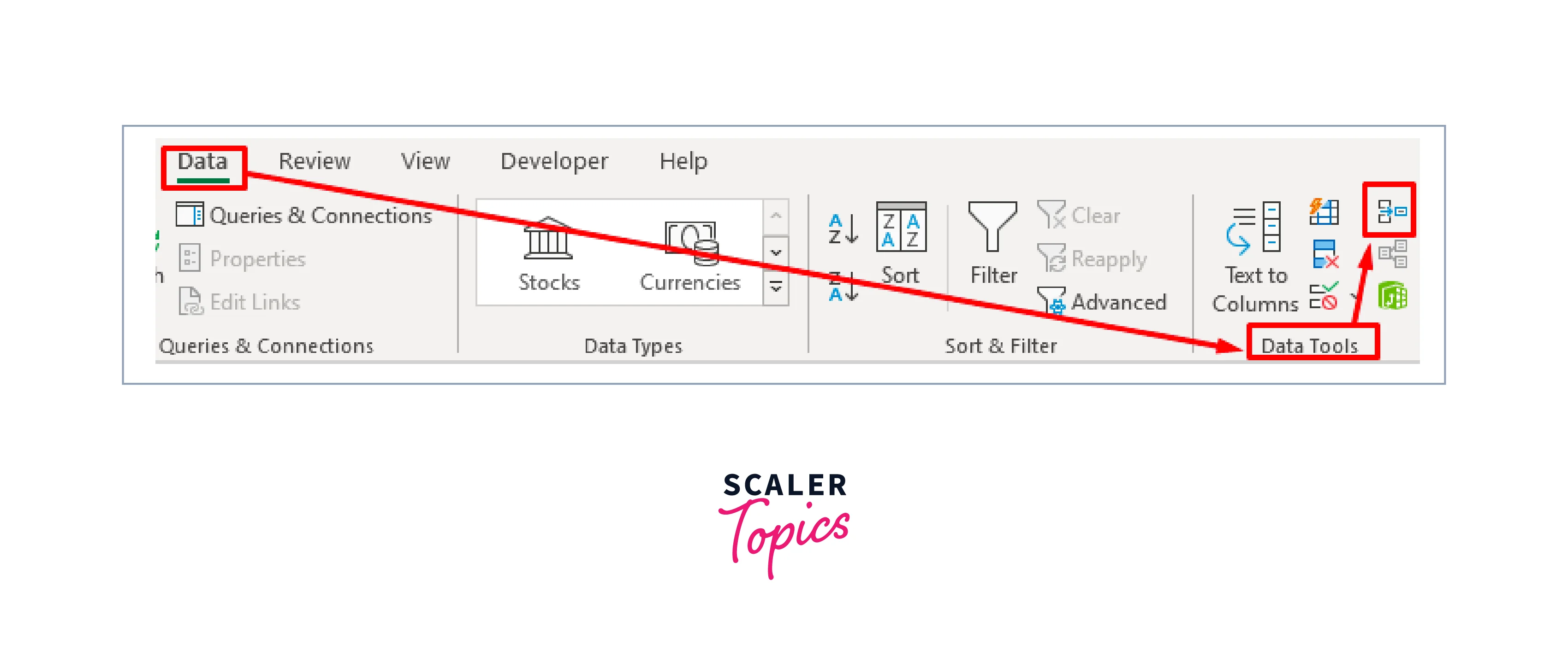
-
Step - 3:
Select the Function you need and Add all the references from the source sheet to the reference box.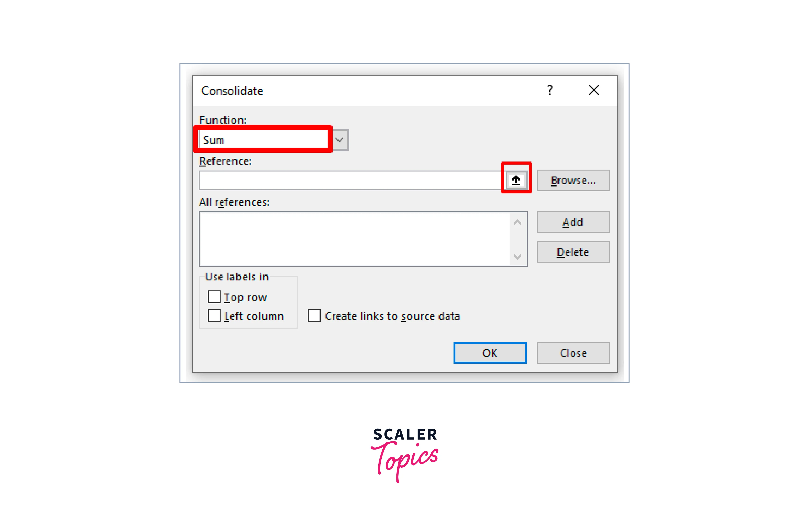
-
Step - 4:
Under the Label box, ensure the check mark is as shown, then click OK.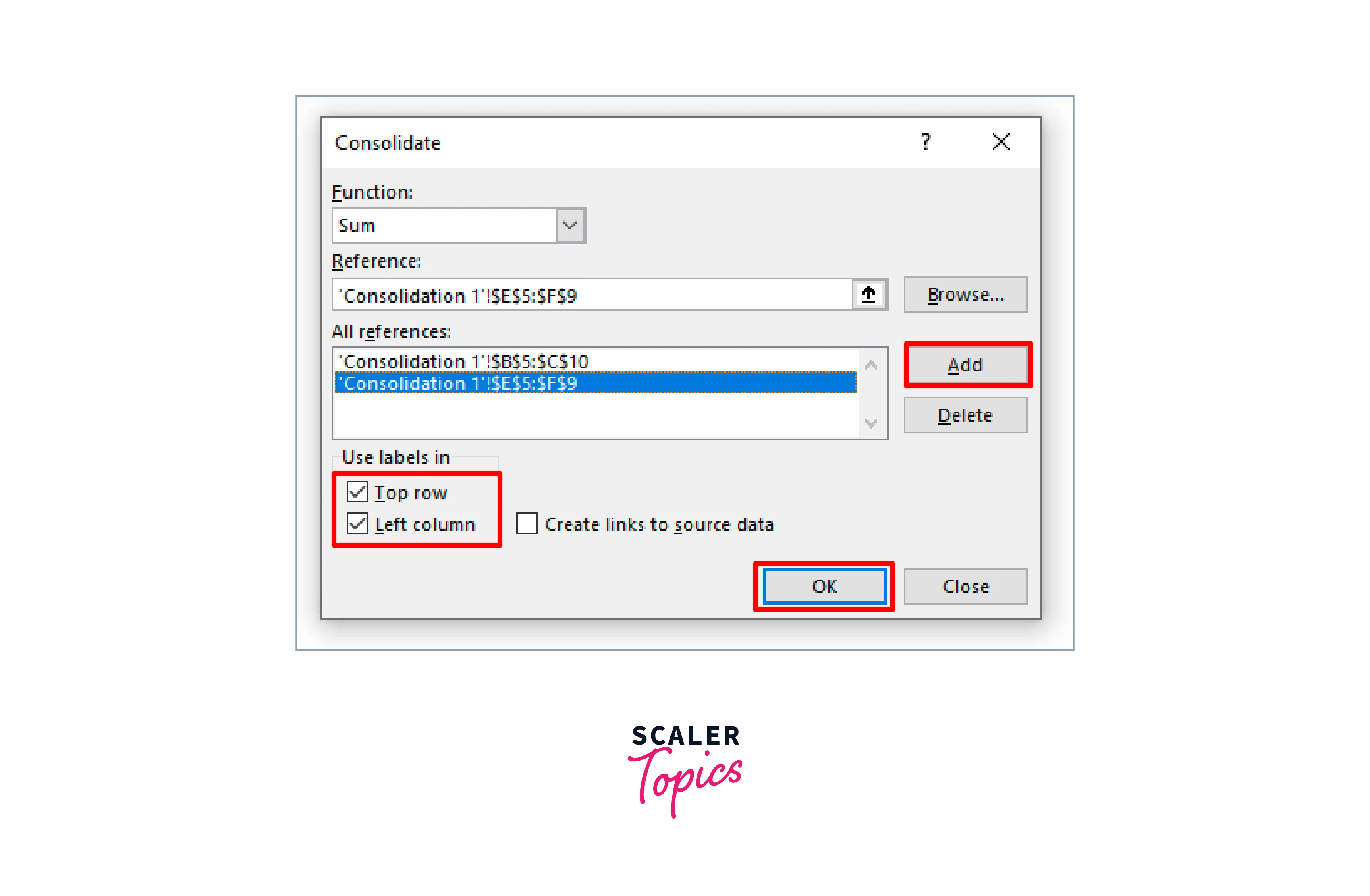
-
Step - 5:
Result will be shown in the destination worksheet.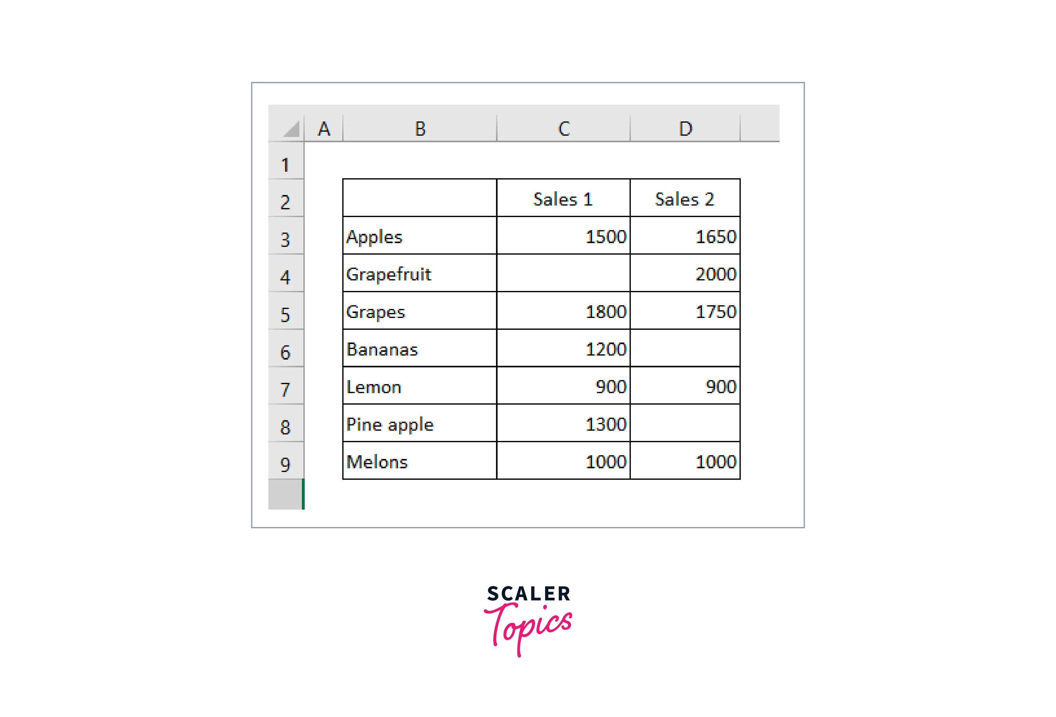
Using Advanced Filter
It is one of the ways to extract the filtered data to another sheet in Excel.
-
Step - 1:
Select the whole dataset.Use the "Ctrl+Shift+L" shortcut to activate AutoFilter.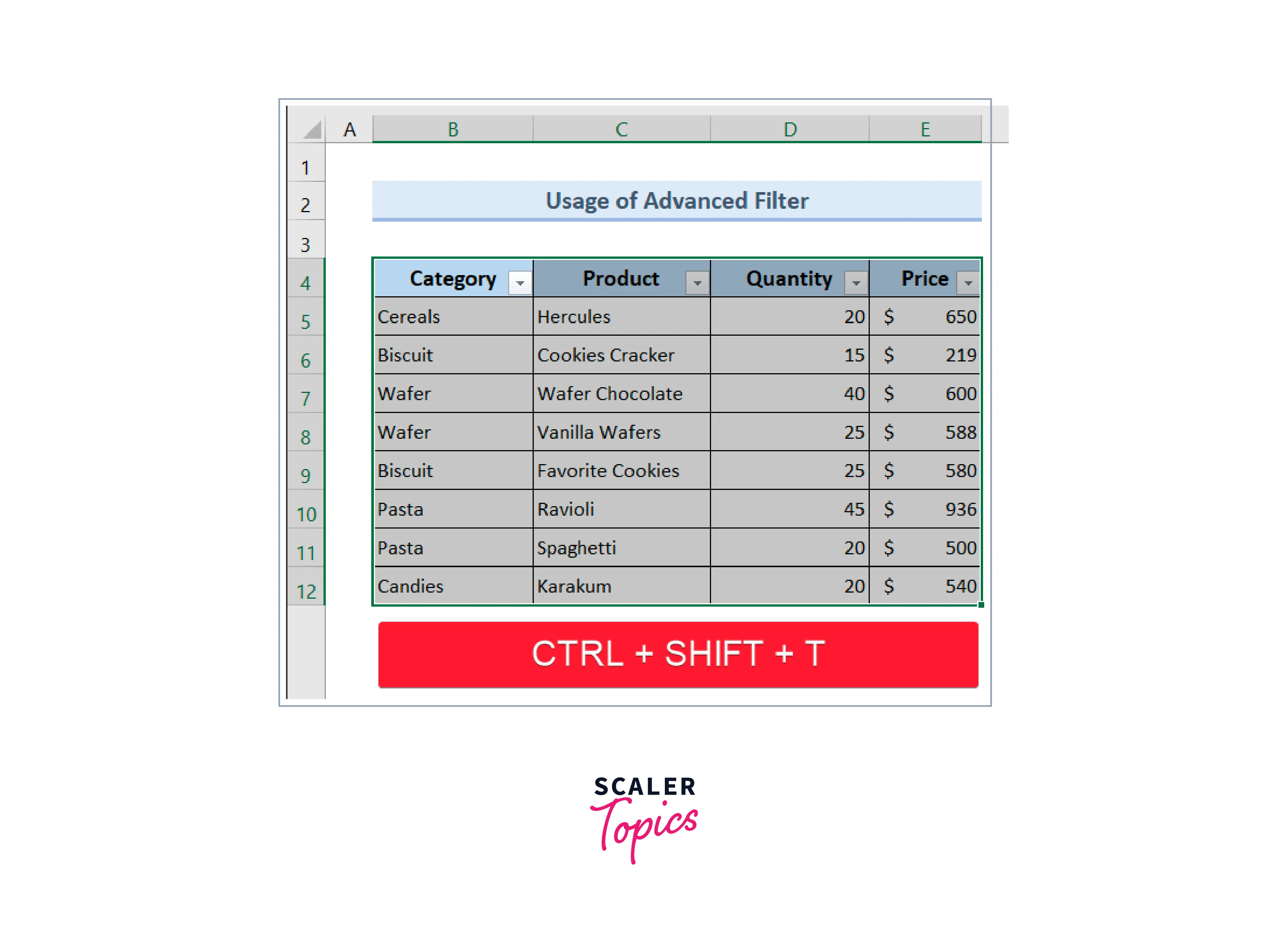
-
Step - 2:
Now, go and open the destination worksheet having criteria. Go to options Data >> Sort & Filter >> Advanced.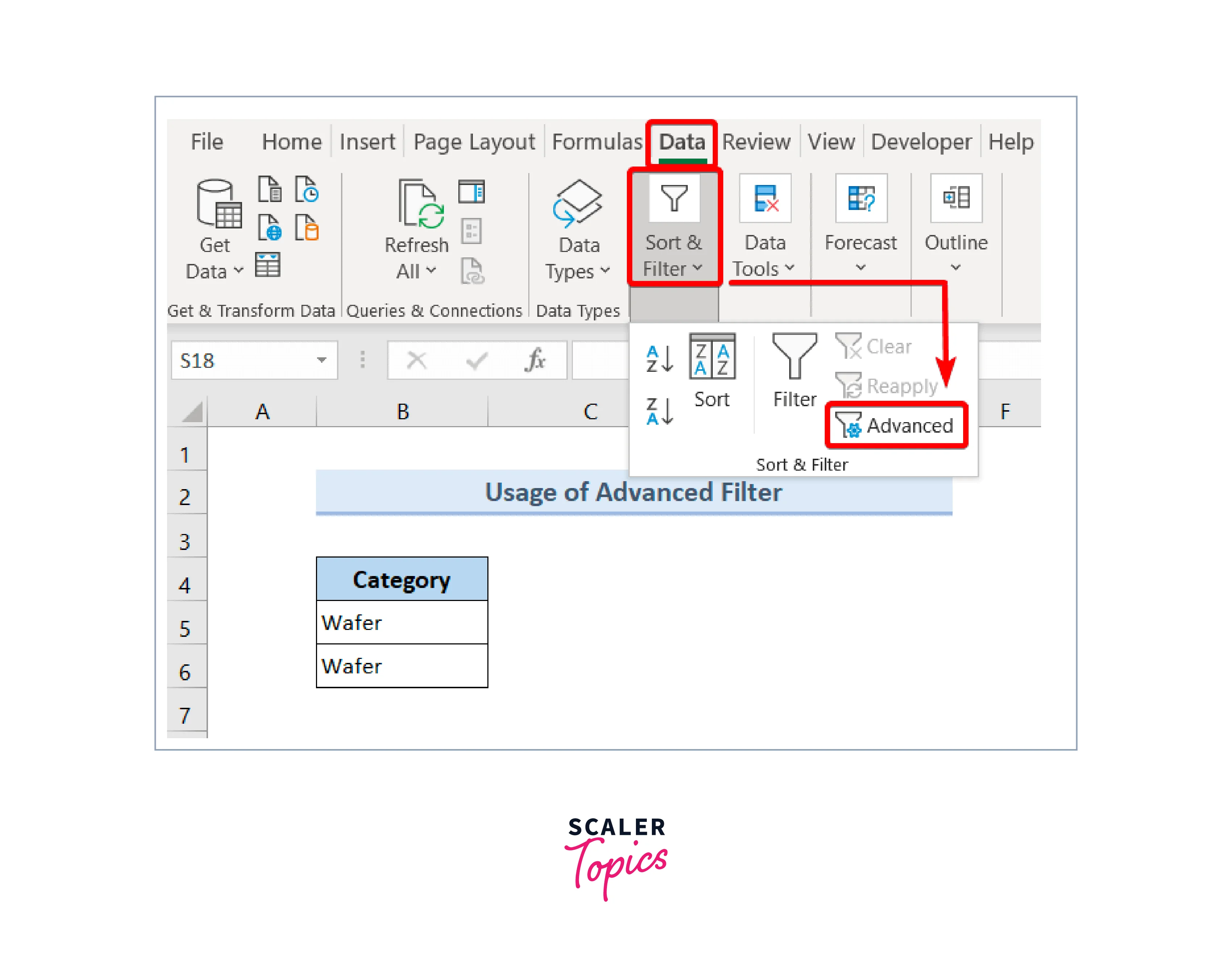
-
Step - 3:
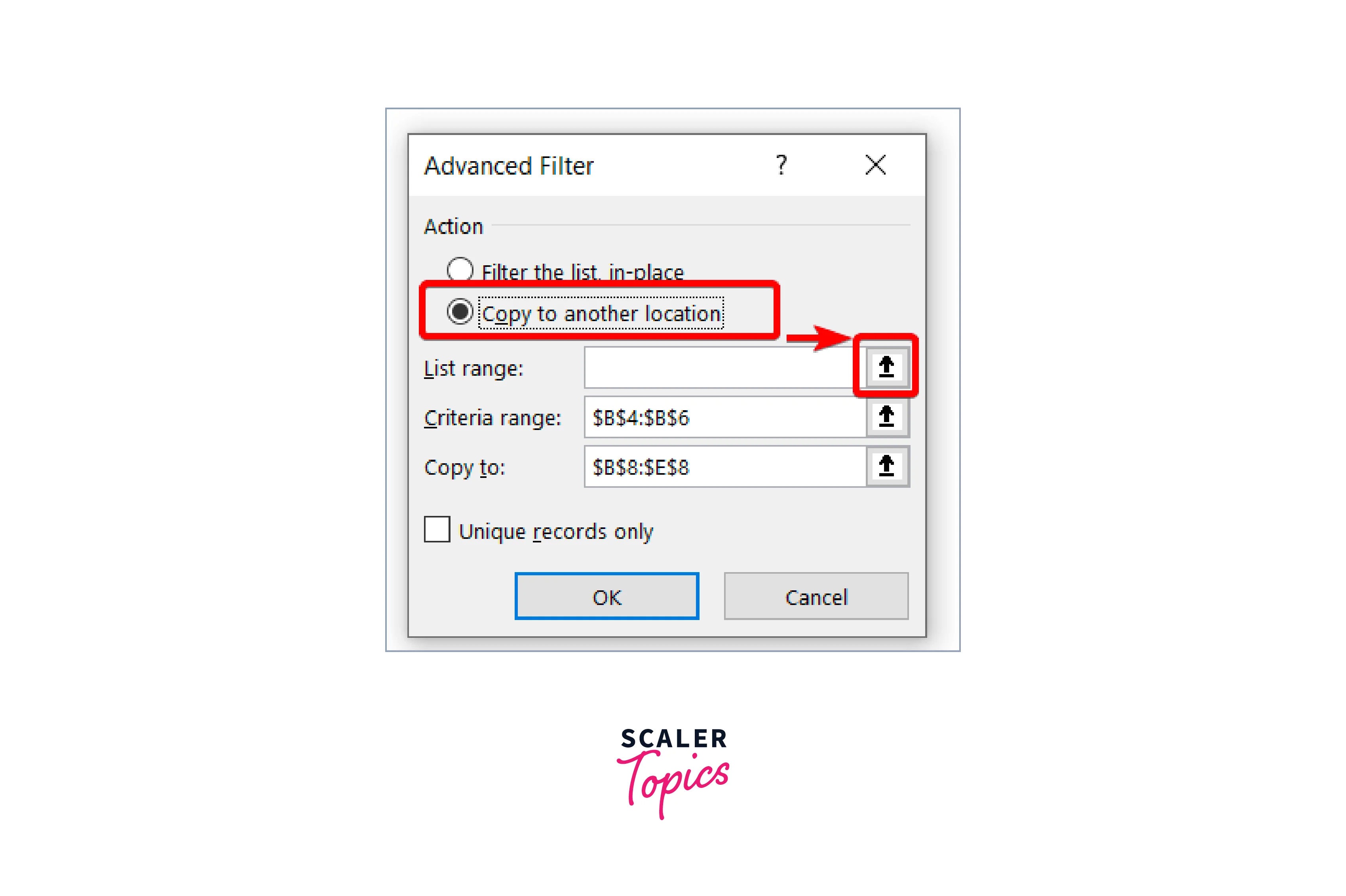
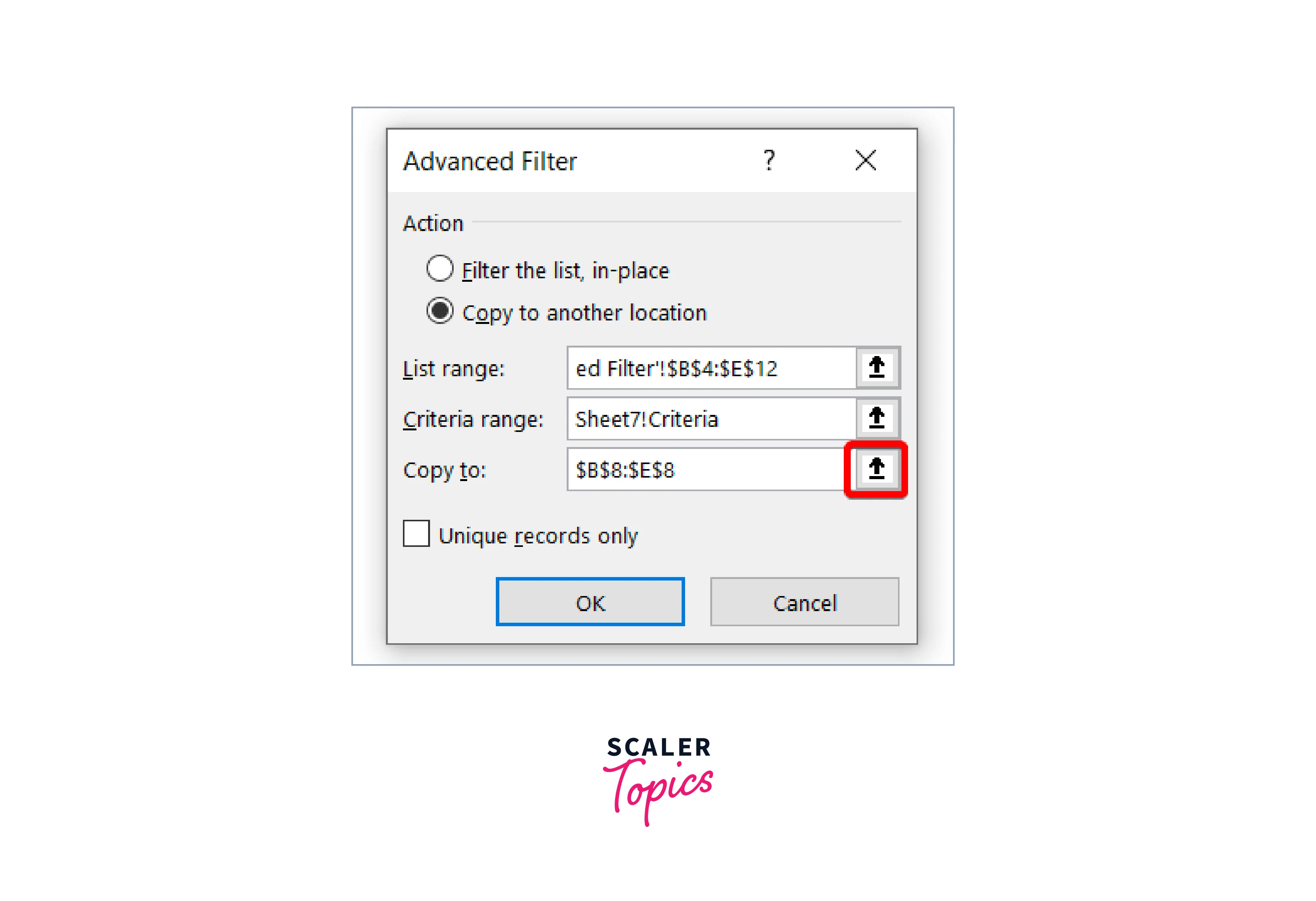
In the Advance Filter dialog box,Under the Action section, choose Copy to another location and click on the Up arrow icon as shown.
-
Select the whole dataset from the original dataset for the List Range.
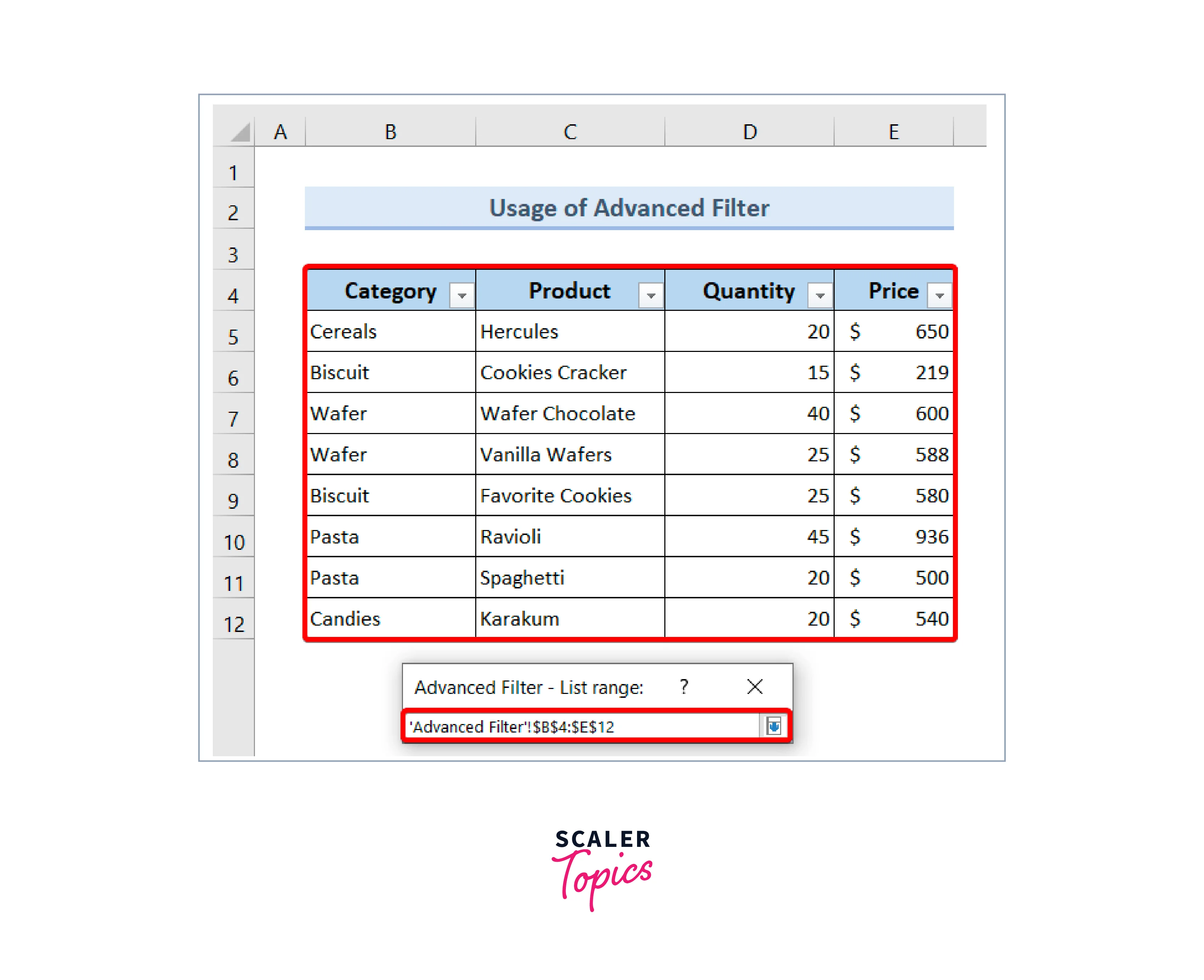
After selecting all data for the listed range, click on the down arrow key from the Advanced Filter – List range dialog box to return.
-
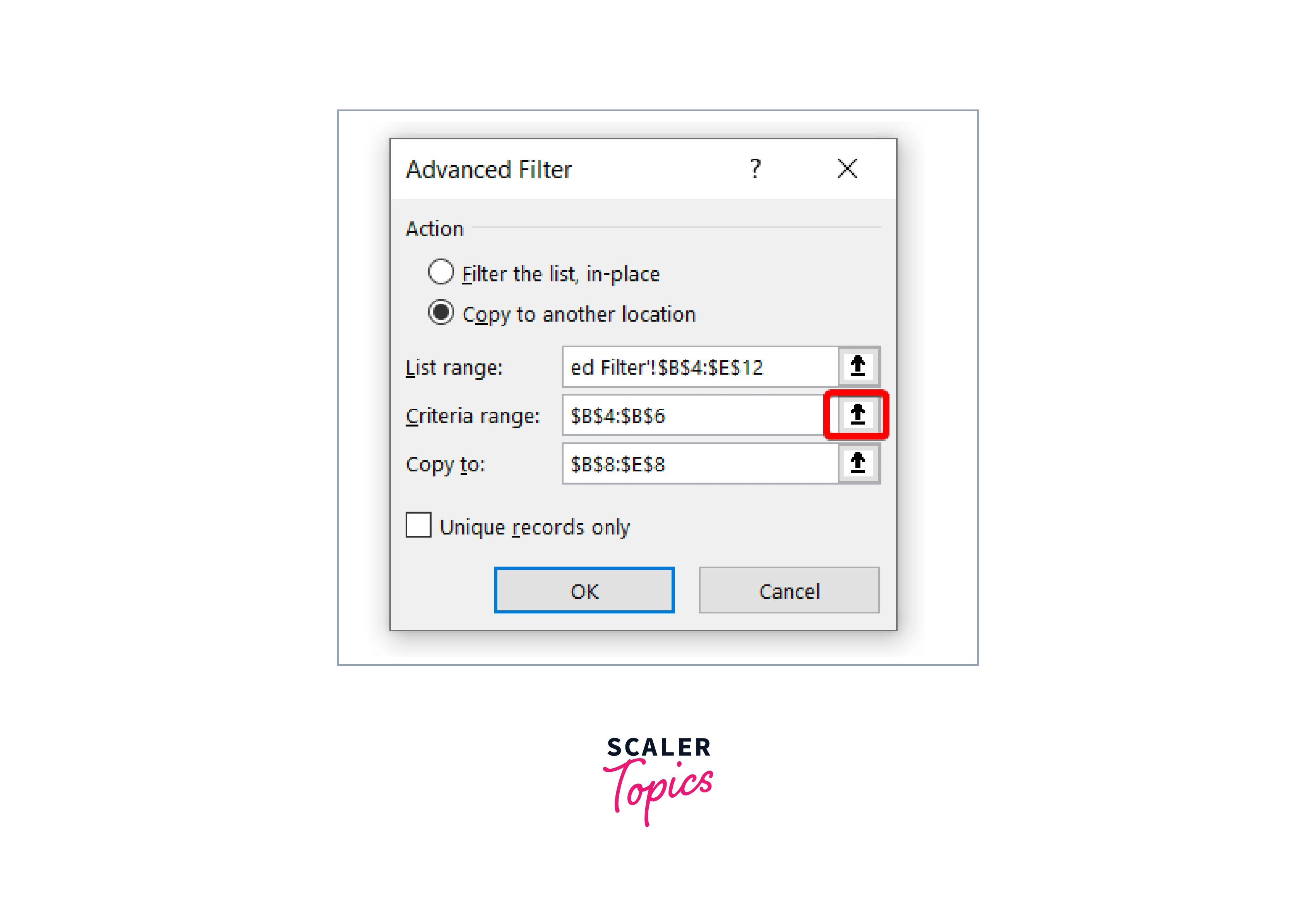
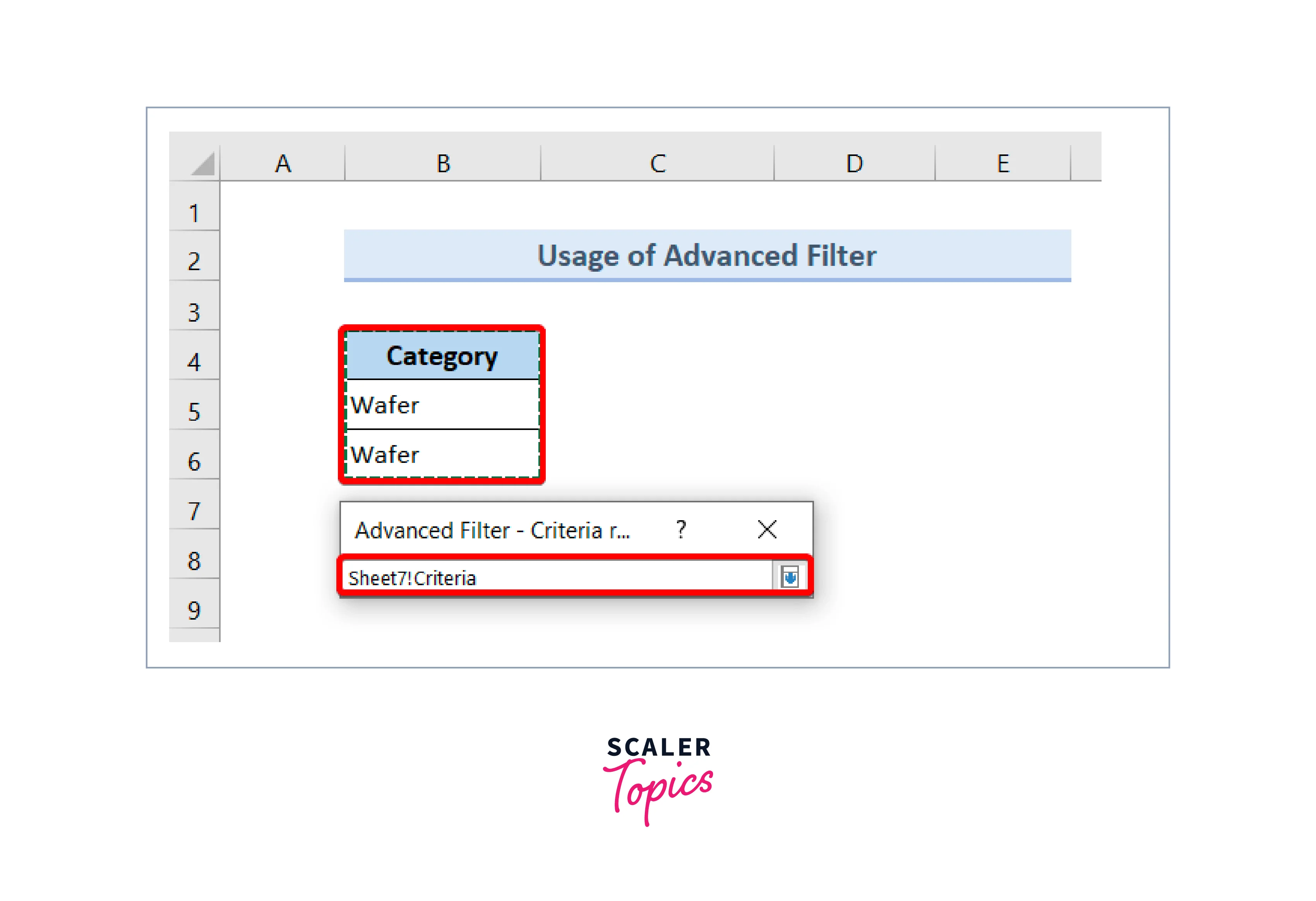
Next, click on the up arrow icon in the Criteria range.
-
For the Criteria range, select the cell range. Then, click on the down arrow icon from the "Advanced Filter – Criteria range" to return.
-
Click on the up arrow key at the Copy to bar at the end of Advanced Filter.
-
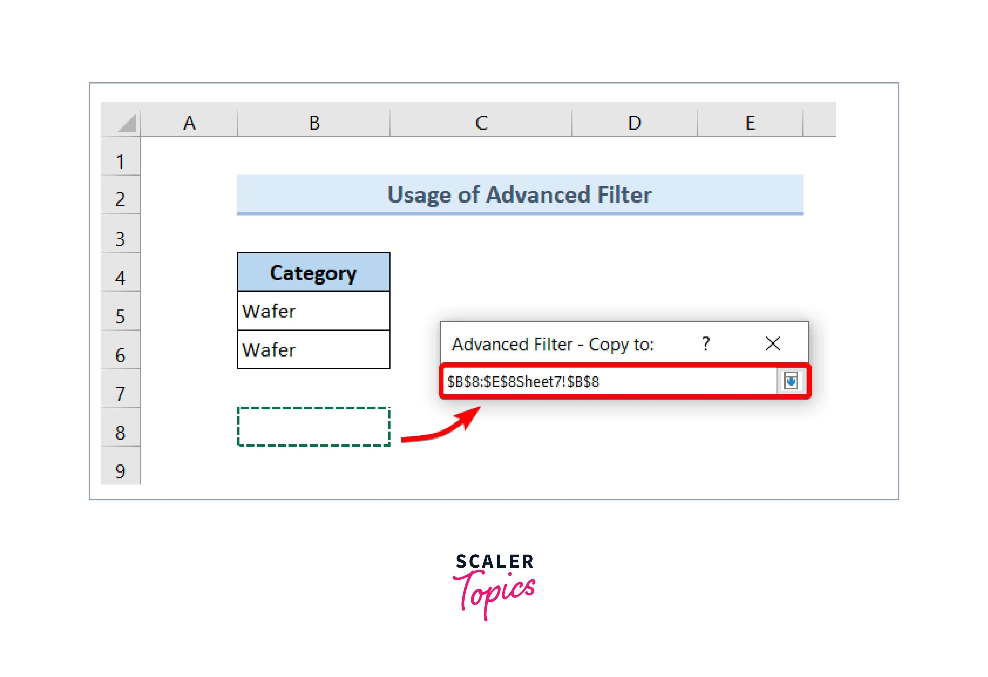
Open the destination worksheet and select a cell to store the filtered data.
-
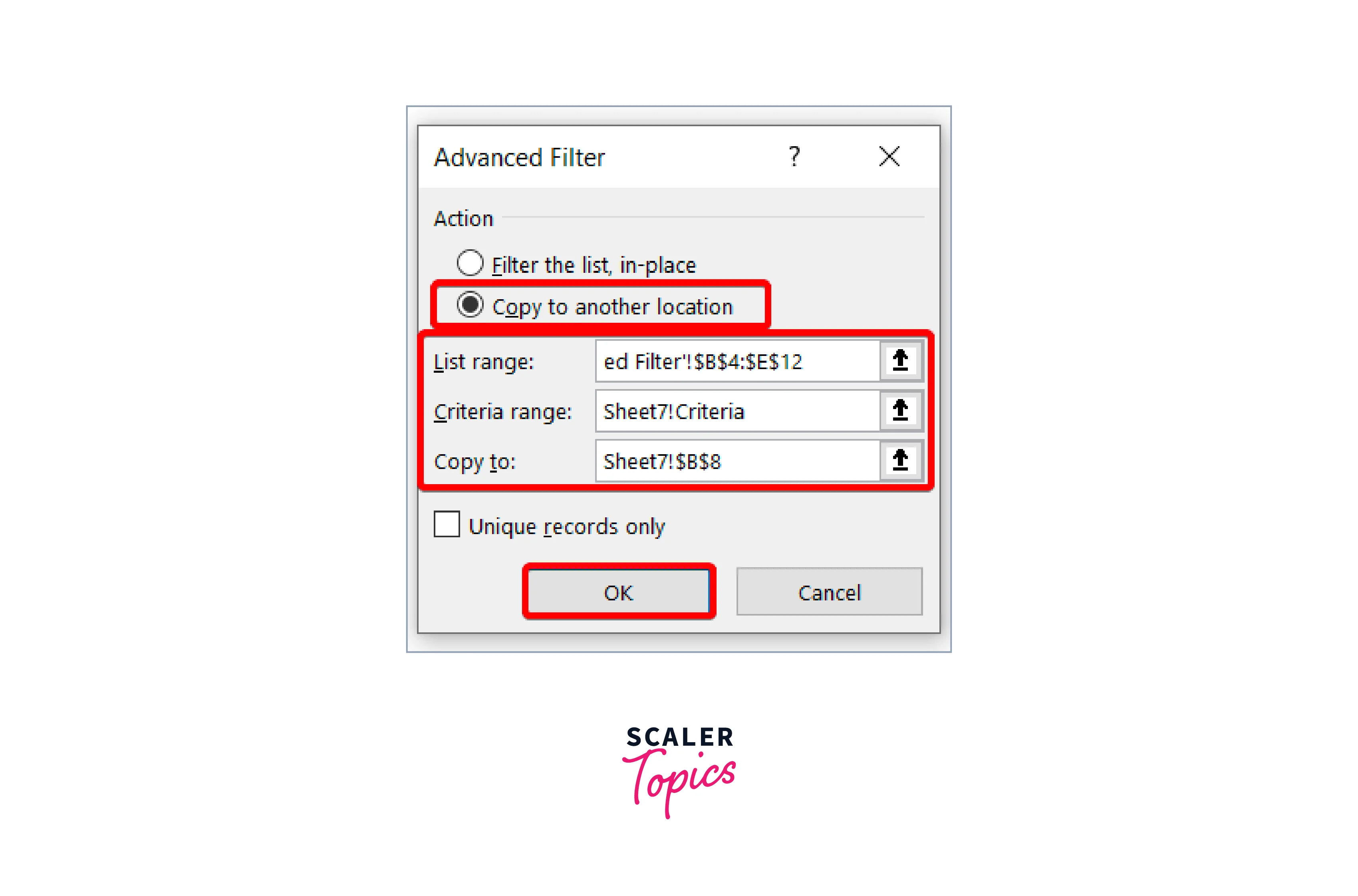
Then click on the down arrow icon from the Advanced Filter and leave the Filter section. Before exiting, check everything is done in the Advanced Filter dialog box and hit OK.
-
-
Step - 4:
Result will be shown in the destination worksheet.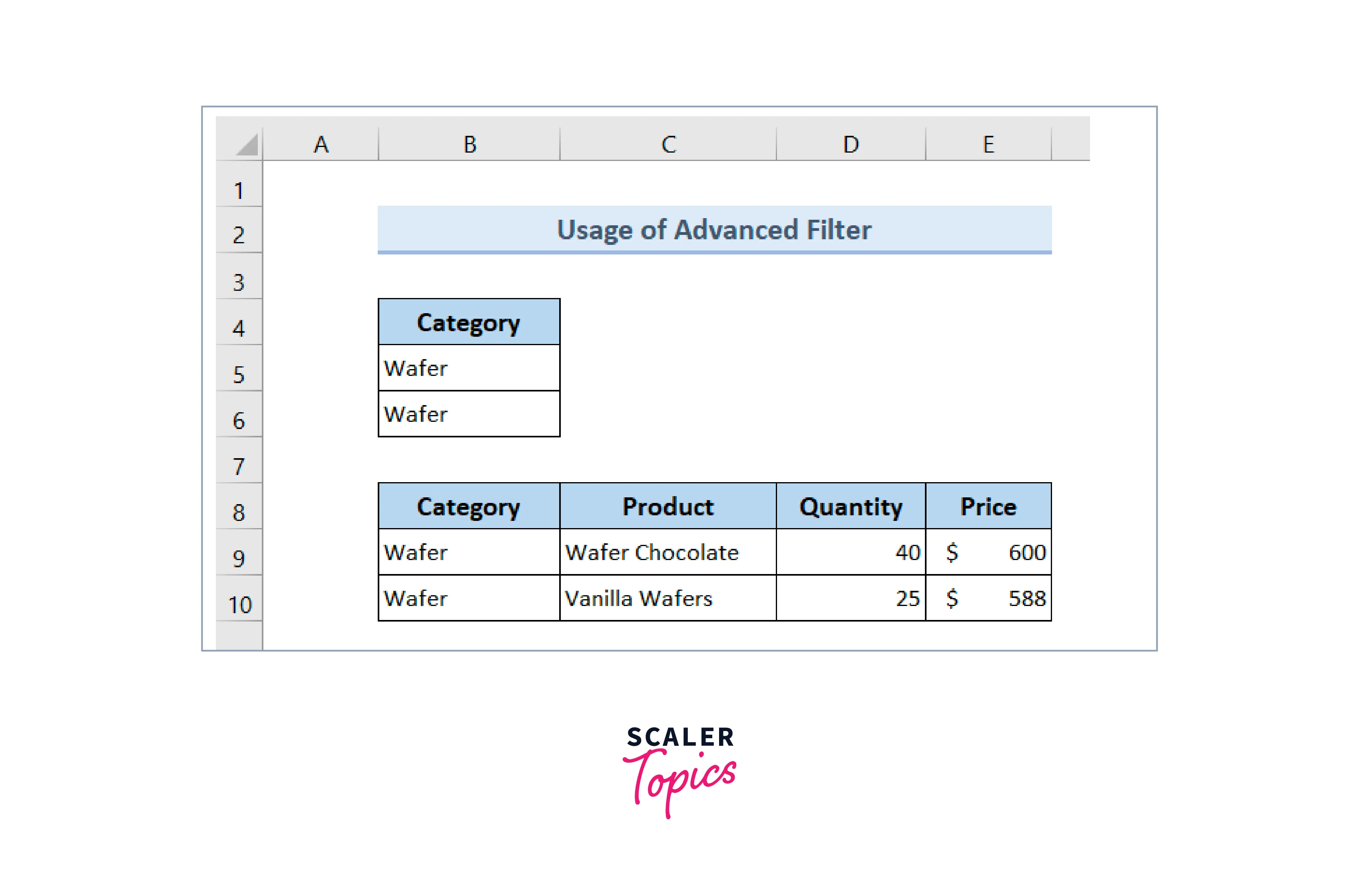
Conclusion
- Data extraction is critical in analyzing and making sense of large amounts of information stored in Excel sheets.
- Various methods can extract data from Excel sheets, including Vlookup, INDEX, INDEX-MATCH, data consolidation tools, and advanced filter tools.
- Vlookup is a useful function that can search for a specific value in a table and return a corresponding value from the same row.
- INDEX is another function that can extract data from a table by returning the value at a specific row and column.
- INDEX-MATCH is a combination of the INDEX and MATCH functions and can be used to search for a specific value in a table and return the corresponding value from the same row or column.
- Data consolidation tools can combine data from multiple sheets or workbooks into one location.
- The advanced filter tool can filter data based on specific criteria and extract only the relevant information.
- These methods are useful in simplifying complex data sets and making them more manageable and accessible.
- By using these techniques, users can save time and effort in extracting data from Excel sheets.
In conclusion, data extraction is an essential process in analyzing and interpreting data, and using the right methods can make this task more efficient and effective.
