How to Freeze Rows and Columns in Excel?

Overview

It might be challenging to stay organized while dealing with a lot of spreadsheet data on your laptop. When working with a small subset of data, we compare two or ten rows of data, but when more rows are involved, things become difficult. There is just one thing you can do when your spreadsheets get too big: How to freeze rows in Excel?

How to Freeze Rows in Excel or Columns?

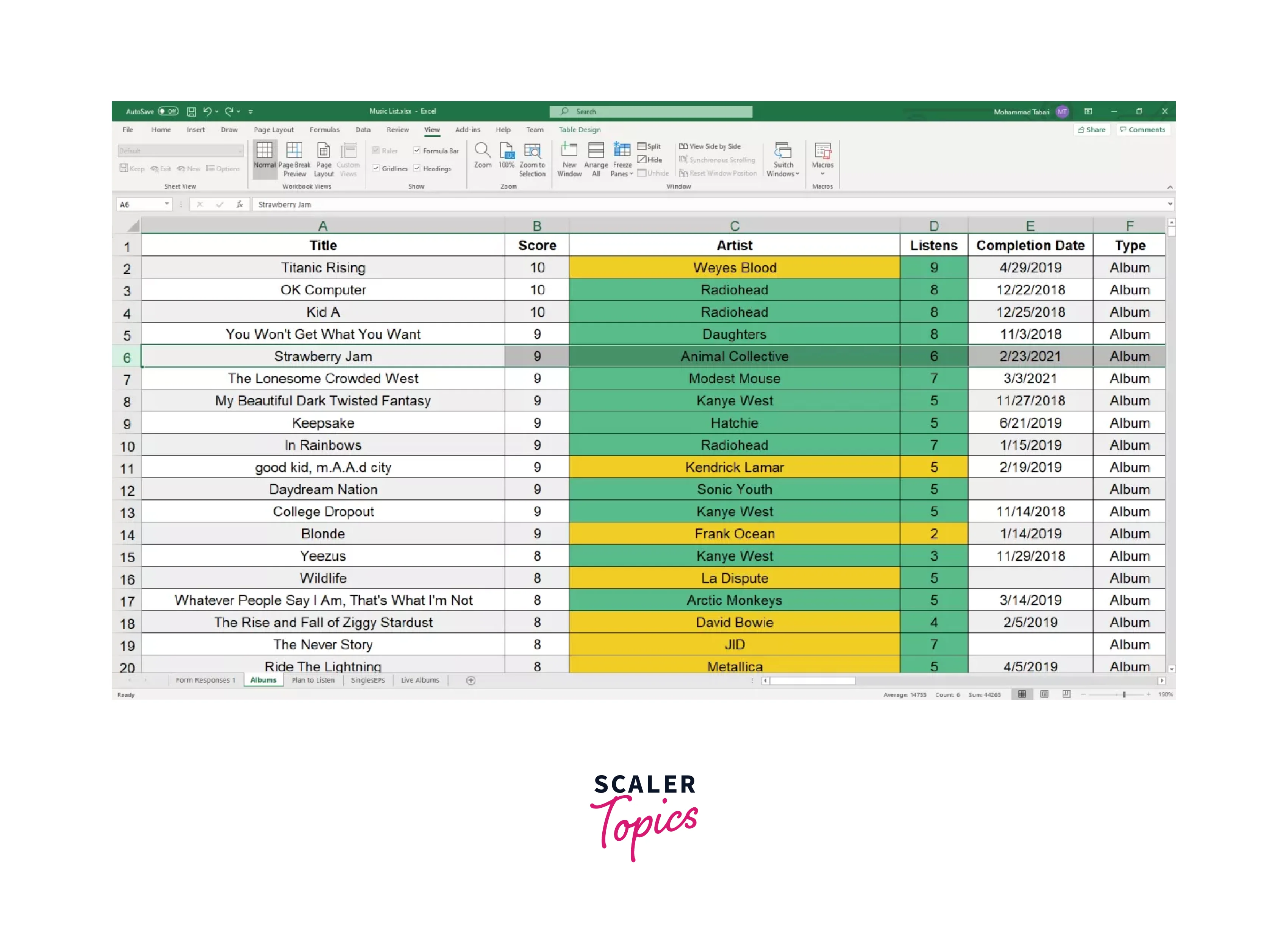
To freeze a row/col or rows/cols, choose the one immediately below. Choose the cell directly adjacent to the column you wish to freeze to do so. In this instance, row 6 has been chosen because we want to freeze rows 1 through 5.
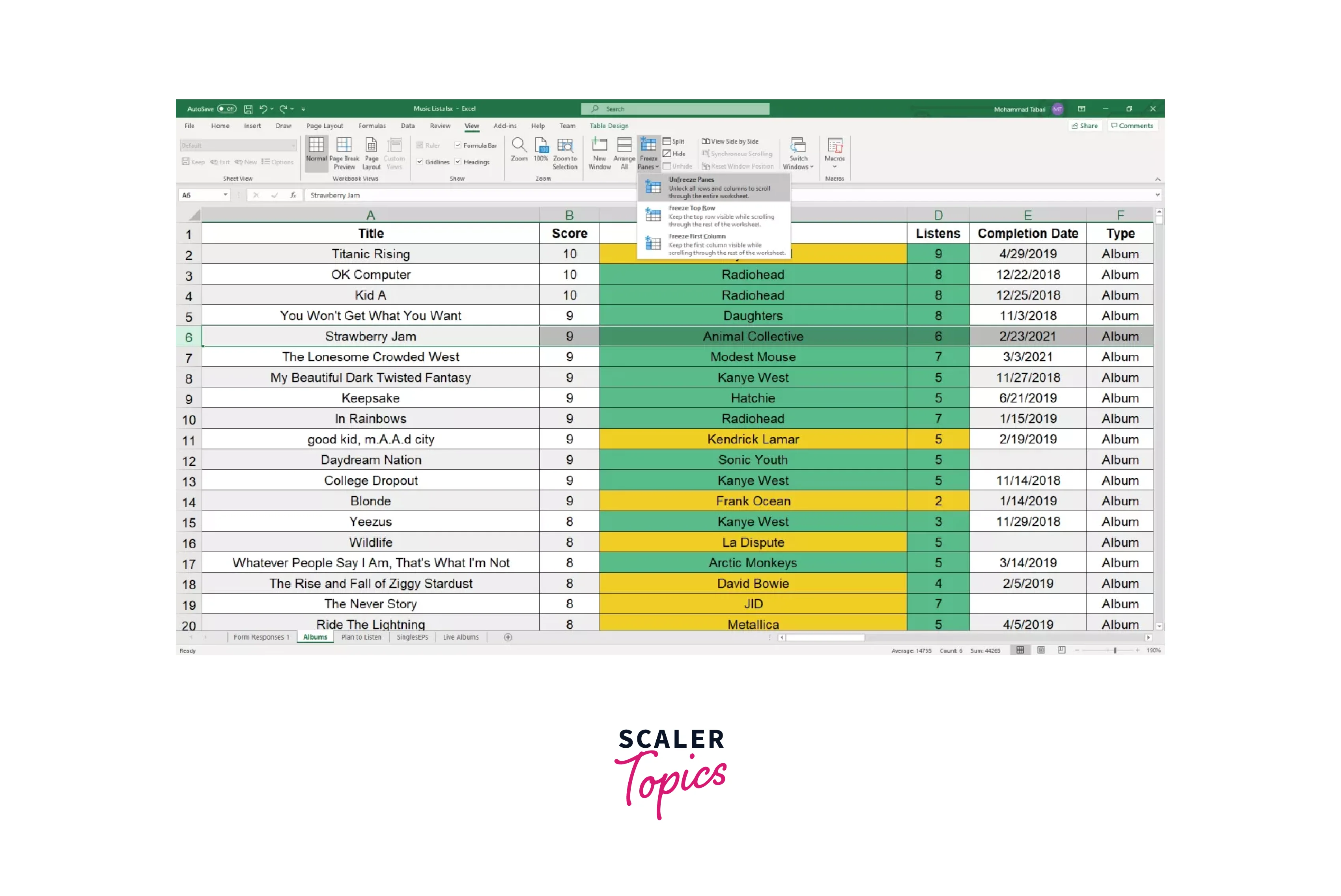
Activate the View tab. This is situated between "Review" and "Add-ins" at the very top.
Click "Freeze Panes" after selecting the Freeze Panes option. The same area where "New Window" and "Arrange All" are located also contains this option.

That's it. In our case, you can see that when you scroll down, the frozen rows or columns remain visible. The green line separating the frozen rows from the ones below them indicates where the rows were frozen.

freezing rows in excel or columns 2

In case you want to freeze more than one column, this is what you need to do:

Select the column (or the first cell in the column) to the right of the last column you want to lock.
Go to the View tab, and click Freeze Panes > Freeze Panes.

Check the image given below to understand it better.

freezing rows in excel or columns 3

How to Unfreeze Rows or Columns?

Return to the Freeze Panes command and select "Unfreeze Panes" to unfreeze the rows or columns.
Additionally, you can also select "Freeze Top Row" or "Freeze First Column" under the Freeze Panes command to freeze the visible top row and any rows above it or to keep the leftmost column visible when scrolling horizontally.
The freeze panes function not only enables you to compare several rows in a lengthy spreadsheet, but it also allows you to retain crucial data, like table headings, permanently in the display.

Conclusion

To Freeze rows or columns, Activate the View tab. This is situated between "Review" and "Add-ins" at the very top. Click "Freeze Panes" after selecting the Freeze Panes option.
To Unfreeze rows or columns, return to the Freeze Panes command and select "Unfreeze Panes" to unfreeze the rows.
Additionally, you can also select "Freeze Top Row" or "Freeze First Column" under the Freeze Panes command to freeze the visible top row and any rows above it.
The freeze panes function not only enables you to compare several rows in a lengthy spreadsheet, but it also allows you to retain crucial data.

FAQs

Q. How can I use this to compare information?

A. For freezing a row below the header, follow the same procedures. For example, choose row 13 and choose Freeze Panes to compare rows 12 and 87. Row 12 will remain visible when you navigate down to row 87 since everything above row 13 will be frozen.

Q. How to freeze multiple columns in Excel?

A. Here is what you need to do if you want to freeze more than one column: Choose the column to the right of the last column you want to lock or the first cell in the column, whichever is appropriate. Click Freeze Panes > Freeze Panes under the View tab.

Q. How to freeze multiple rows in Excel?

A. Choose the row beneath the last row you want to freeze, pick the View tab, and then click Freeze Panes to lock multiple rows (beginning with row 1). Choose the column to the right of the final column you want to freeze, pick the View tab, and then click Freeze Panes to lock several columns.