Building a GAN from scratch

Introduction

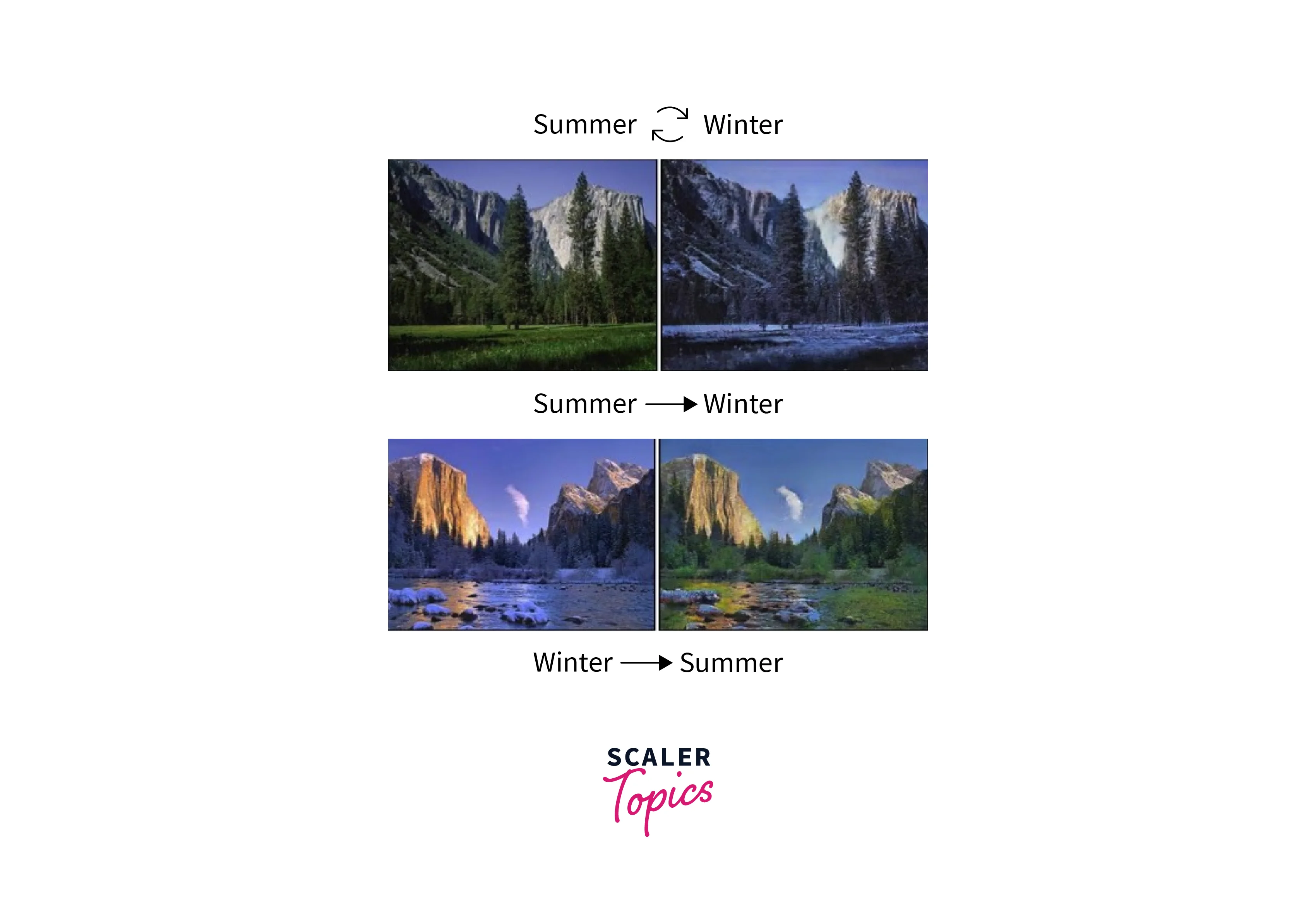
A GAN, or Generative Adversarial Network, is a neural network we can use to generate new, previously unseen images from a given dataset. GANs have two main parts: a generator network and a discriminator network. The generator network creates new images, while the discriminator network evaluates the images generated by the Generator and tries to distinguish them from the original images in the Dataset. The two networks are trained together in an adversarial manner, with the Generator trying to produce images that can fool the Discriminator and the Discriminator trying to identify the generated images correctly. GANs can be used for various tasks, such as image synthesis, style transfer, and super-resolution. They are usually unsupervised, but many architectures also consider labels during Training. Some examples of outputs GANs are shown here.

GANs have more complex architectural pipelines than a standard Convolutional network. They generally have two major structures, the Generator, and the Discriminator. These structures are Convolutional networks that we can substitute for other networks that perform similar functions.

The training paradigm for GANs is called Adversarial Training and relies on an interplay between the Generator and the Discriminator.

This article will examine a Generative Adversarial Network and its components. After we understand the parts, we will build our own GAN from scratch and train it on a dataset of handwritten images (MNIST).

Architecture of a GAN

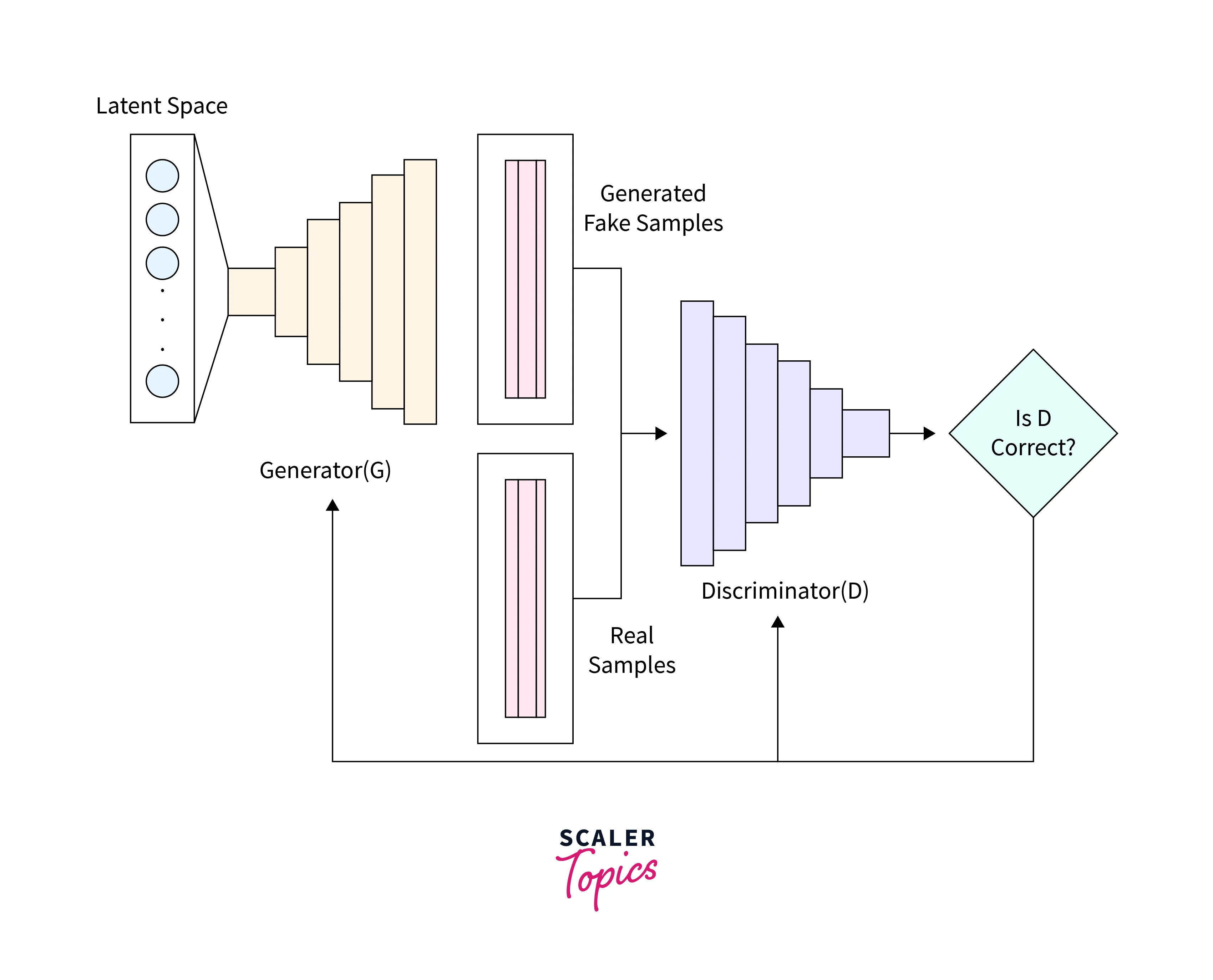
A GAN's architecture is unique in that it comprises two neural networks, the Generator and the Discriminator, that work together to create new, previously unseen images from a given dataset. These two networks are trained in an adversarial manner, with the Generator trying to produce images that can fool the Discriminator and the Discriminator trying to identify the generated images correctly.

Consider the architecture diagram shown below.

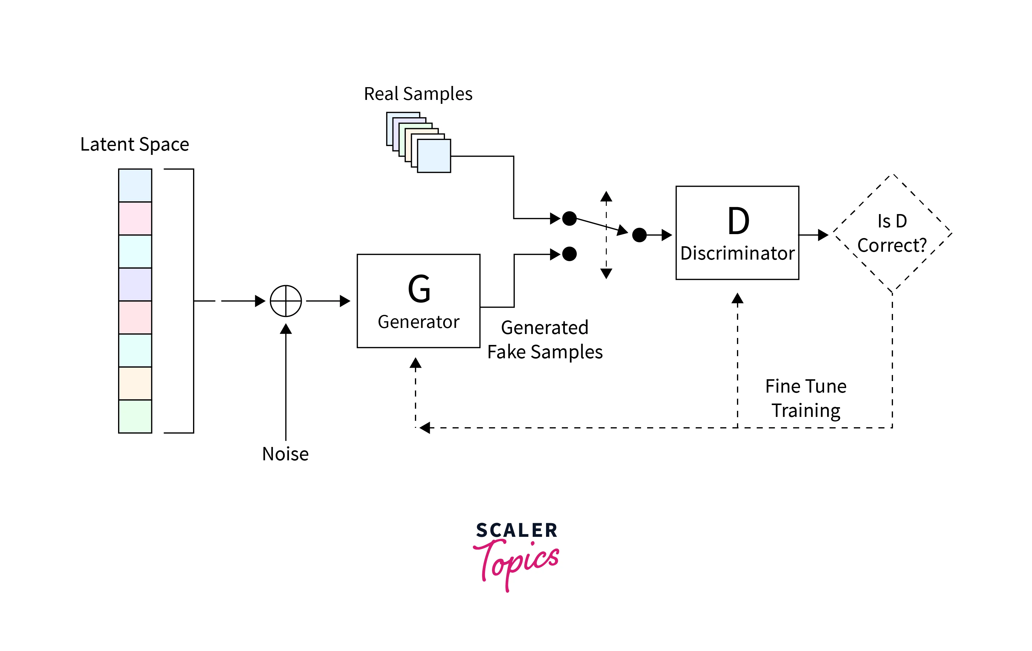
The first part of the architecture is the Generator, whose job is to create images realistic enough that the Discriminator cannot tell the difference between a fake image and a real one.

Generator

The generator network is responsible for creating new images. It takes a random noise as input and transforms it into a realistic image. The generator network is a simple neural network composed of blocks of fully connected linear layers and Leaky ReLU activations. These layers help learn features of the Dataset and create an image similar to the real images.

In the final layer of the Generator, the Leaky ReLU activation is replaced by a Tanh activation. The Tanh activation function is used because it maps the output of the Generator to the range of (-1,1), which is the range of the MNIST data images. This range is because the Generator should output an image similar to the real images. Squishing the generated image to the range of the real image makes it more similar to the real image.

This mapping to the range of the real images also helps produce images that are not just random noise but are closer to the real images in terms of features and overall structure. This mapping makes the Generator more robust and effective in producing realistic images.

Discriminator

The discriminator network is the second part of a GAN architecture, and its main role is to evaluate the images generated by the Generator and determine the probability that the image is real. The Discriminator is a binary classifier that returns the probability of the image being real or fake. It comprises a series of fully connected linear layers, Leaky ReLU activations, and Dropout layers. The fully connected linear layers in the discriminator network help learn the features of the real images, while the Leaky ReLU activations help prevent the gradients from becoming zero. The Dropout layers are used to prevent overfitting, which is a common problem in deep neural networks. The final layer of the discriminator network is a block with an FC layer and a Sigmoid activation function. The Sigmoid function maps the output to a probability between 0 and 1. The output of the Sigmoid function is the probability that the image is real, which is what the Discriminator is trying to determine. The Discriminator's goal is to correctly identify the generated images as fake and the real images as real; this way, the Generator will improve its ability to produce more realistic images.

Demystifying the Loss Function

Loss functions are an essential part of any neural network pipeline. Before we learn how to make a Generative Adversarial Network, we must first understand the loss functions.

Discriminator loss

The Discriminator's job is to classify the generated images into real or fake and return the probability that it is real. To do so, it needs to do extremely well at ensuring that the input it gets belongs to the real Dataset. It should also ensure that if the input is fake, it is not classified as belonging to the real Dataset. Mathematically, this can be understood as maximizing $D(x)$ and minimizing $D(G(z))$.

Generator loss

The Generator is tasked with ensuring that the Discriminator is fooled. It can do so by creating realistic images that the Discriminator thinks are real. This process can be thought of as ensuring that the Discriminator classifies an image sampled from the fake Dataset as belonging to the real one. Mathematically, this is formulated as maximizing $D(G(z))$. Using this as the loss might make the network extremely confident, even if it is wrong. To prevent this from happening, $log(D(G(z)))$ is used instead.

Total loss

There is no net loss that is used in practice. Still, while learning to make a Generative Adversarial Network, we must consider the total theoretical loss the network is trying to optimize. Training a Generative Adversarial Network is a game between two enemies (aka adversaries). In other words, this is a MinMax game where one party attempts to reduce the probability of the other winning. Both parties are simultaneously also trying to increase their chances of winning. Mathematically, this can be represented as $\underset{G}{min} \underset{D}{max} V(D,G) = \mathbb{E}_{x \sim p_{data}(x)}[log(D(x)] + \mathbb{E}_{z \sim p_{z}}[log(1 - D(G(z))]$

Heuristic loss

Understanding heuristics is another aspect of knowing how to make a Generative Adversarial Network. These heuristics are not part of any network directly but are training guidelines that work for most GANs. (Any GAN created before 2016, at least.) We can use these heuristics to ensure stable reductions in the loss landscape, which is key to training a Generative Adversarial Network well.

• If the network has pooling layers, they can be replaced with stridden convolutions in the Discriminator and fractionally stridden convolutions in the Generator.
• We can use Batch Normalization layers in the Generator and the Discriminator.
• If the architecture is deep, we should remove FC layers for better performance.
• As for activations, the ReLU activation should be used for all the layers. The only exception is the output layer, where a TanH activation should be used.

How to Train a Generative Adversarial Network?

We need an optimization algorithm that performs gradient descent on the network weights to train the GAN. The SGD (Stochastic Gradient Descent) algorithm is used for a vanilla GAN like ours. The Generator and the Discriminator are assigned to their SGD optimizer for Training. This procedure ensures that they both learn independent weights. Since the outputs of both networks flow between other, they are influenced by each other as well.

The general training paradigm for any GAN is as follows. This paradigm is always a good place to refer to when building a Generative Adversarial Network.

• Obtain an image, and create a random noise the same size as the image.
• Pass these images to the Discriminator and obtain the probability of the image passed being real or fake.
• Create another noise the same size as before, and pass it to the Generator.
• Train the Generator with this input data.
• Repeat all the previous steps until the weights are optimized, and satisfactory results are obtained.

Implementing GAN in Python.

In this article, we will create a GAN that can create novel handwritten digits every time it is called. We will take all the concepts we have learned and, finally, learn how to make a Generative Adversarial Network in Python using the Tensorflow library. Before building the network and training pipeline, we must choose a dataset and set up the optimizers and loss functions. After the initial set-up, we can train the network and generate handwritten digits (or any other data).

Imports

First, we import all the required libraries. We will import the plotting library matplotlib and the numerical processing library numpy. In this case, we will import all the required functions from Tensorflow.

Setup Configuration

We need to explore our configuration options to understand further how to make a Generative Adversarial Network. We first define the image size we want to load and generate. Since we are using the MNIST dataset, we set this to 28x28. The MNIST dataset is grayscale, and this only has one channel. We can set the size of the latent space to 100. If the Dataset was more complex, We could choose a higher number.

Dataset

A dataset of handwritten digits is almost ubiquitous in deep learning. The Dataset we use in this article is the Modified National Institute of Standards and Technology database or MNIST. A sample of this Dataset is shown below.

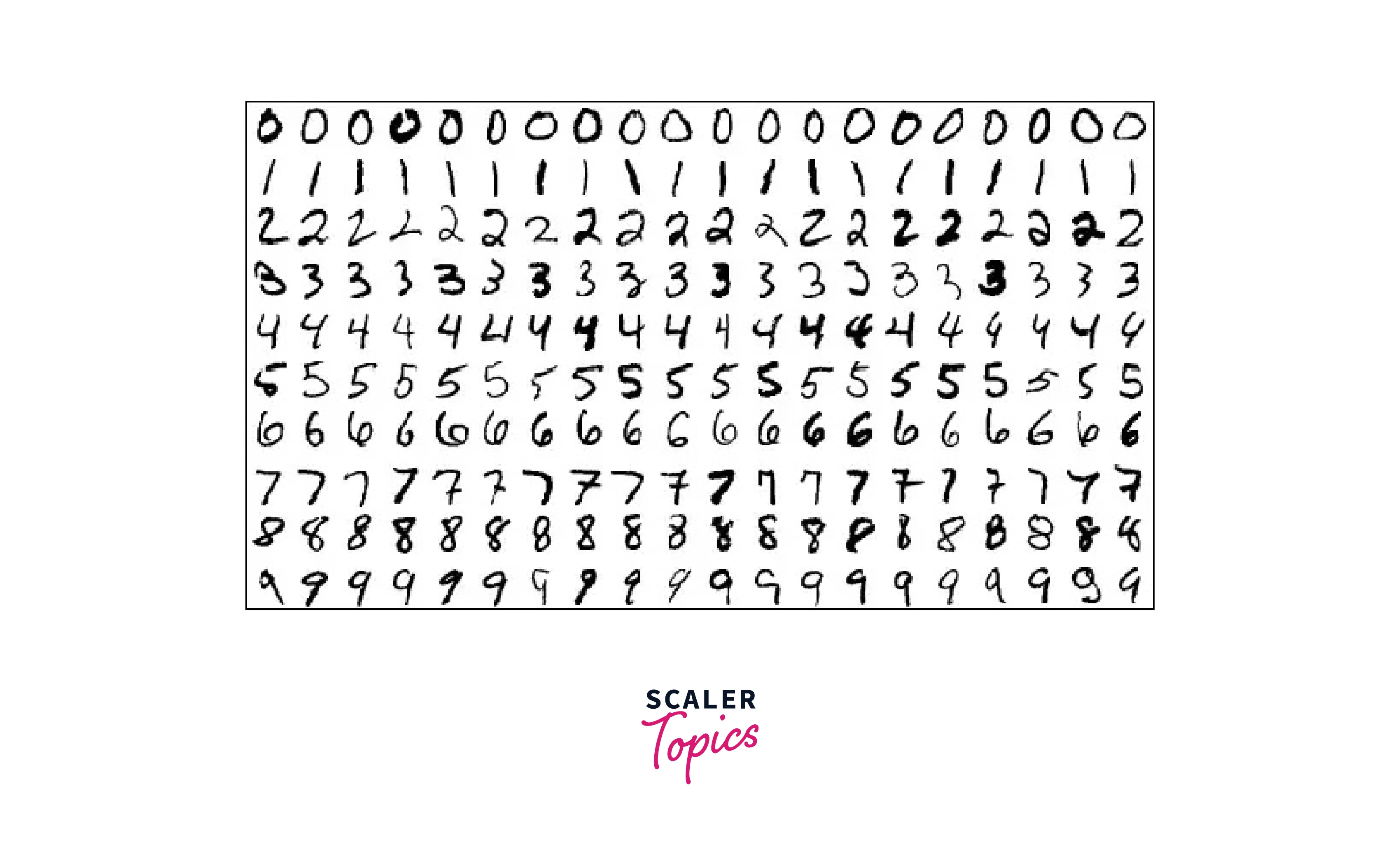
The MNIST is a very simple dataset for modern networks to model, so it is a good challenge for our vanilla GAN.

The MNIST dataset comes pre-installed with Keras, which we can use directly. We need to pre-process the images by normalizing them and converting them to 3 dimensions to pass them to the network (a Generative Adversarial Network cannot directly process 2D images without changing the architecture). We also create proxy containers for the real and fake images to save memory during Training.

Networks

We now look at the network architecture to understand how to make a Generative Adversarial Network from scratch.

Discriminator

To create the Discriminator, we define a function that returns a model with the network defined. This function does not compile the model as we need to call it multiple times, and pre-compiling it will lead to issues when we do.

Generator

The Generator is built similarly to the Discriminator. We define a custom function to create the Generator but do not compile it for now. The noise is also generated and passed through the network here.

Optimization

We define the following functions to set up the optimizers for both networks. We will be using an SGD optimizer in this case for both models.

Training

Before we can train, we need to define a few utility functions. The first function sets up both the Generator and the Discriminator for Training. It compiles the combined model and also creates noise.

The entire training loop is then as follows. This loop follows the exact procedure described in previous sections. We also add a running counter that tells us how far along we are in Training and saves the outputs every sample_interval epochs.

After defining these functions, we train it for as many epochs as possible. For the sake of this article, we can train it for 10,000 epochs. Longer epochs do not necessarily mean better performance.

Testing

We also need a function that samples a batch of data to generate images on demand during/after Training. This function creates a random noise vector and uses the trained Generator to perform a prediction on the noise. The generated images are then plotted for a batch of images.

In the training loop, if the number of passed epochs is a multiple of the sample interval (how many epochs to skip before saving the outputs), we call this function and save the images. We can also do this later on.

Results

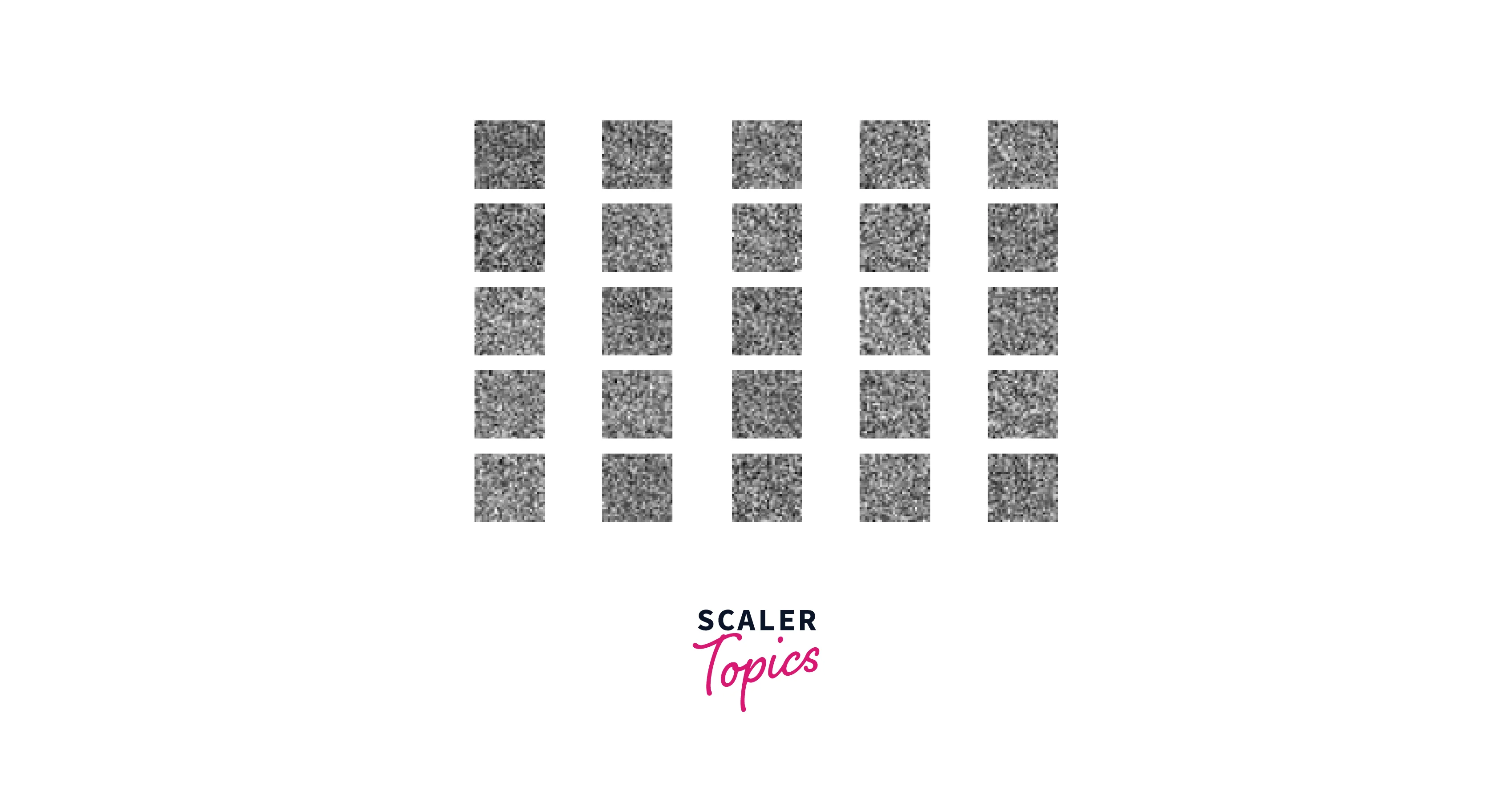
The code we wrote saves images at an interval of 200 epochs. For clarity, we can look at the images generated at the start, at 400 epochs, at 5000 epochs, and finally, after 10,000 epochs.

At the start, we have random noise.

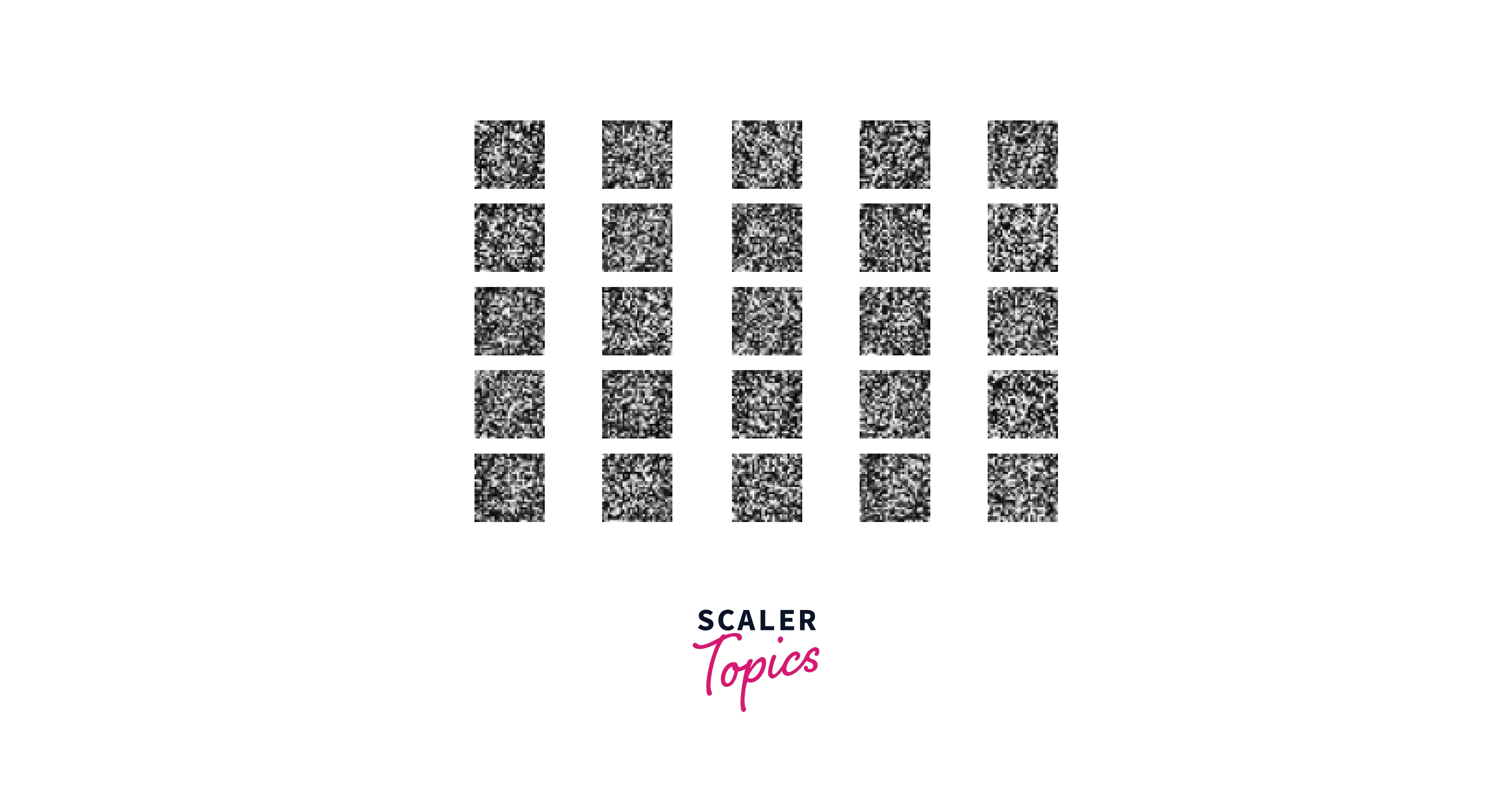
After 400 epochs, we are getting somewhere slowly. But these results are different from real digits.

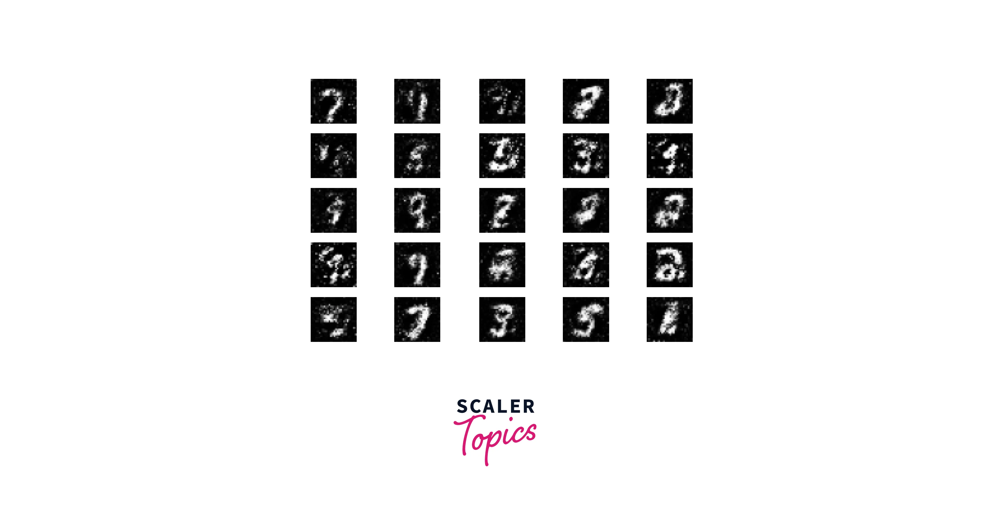
After 5000 epochs, we can see figures that resemble the MNIST dataset. We get the following outputs after training the network for the entire 10,000 epochs.

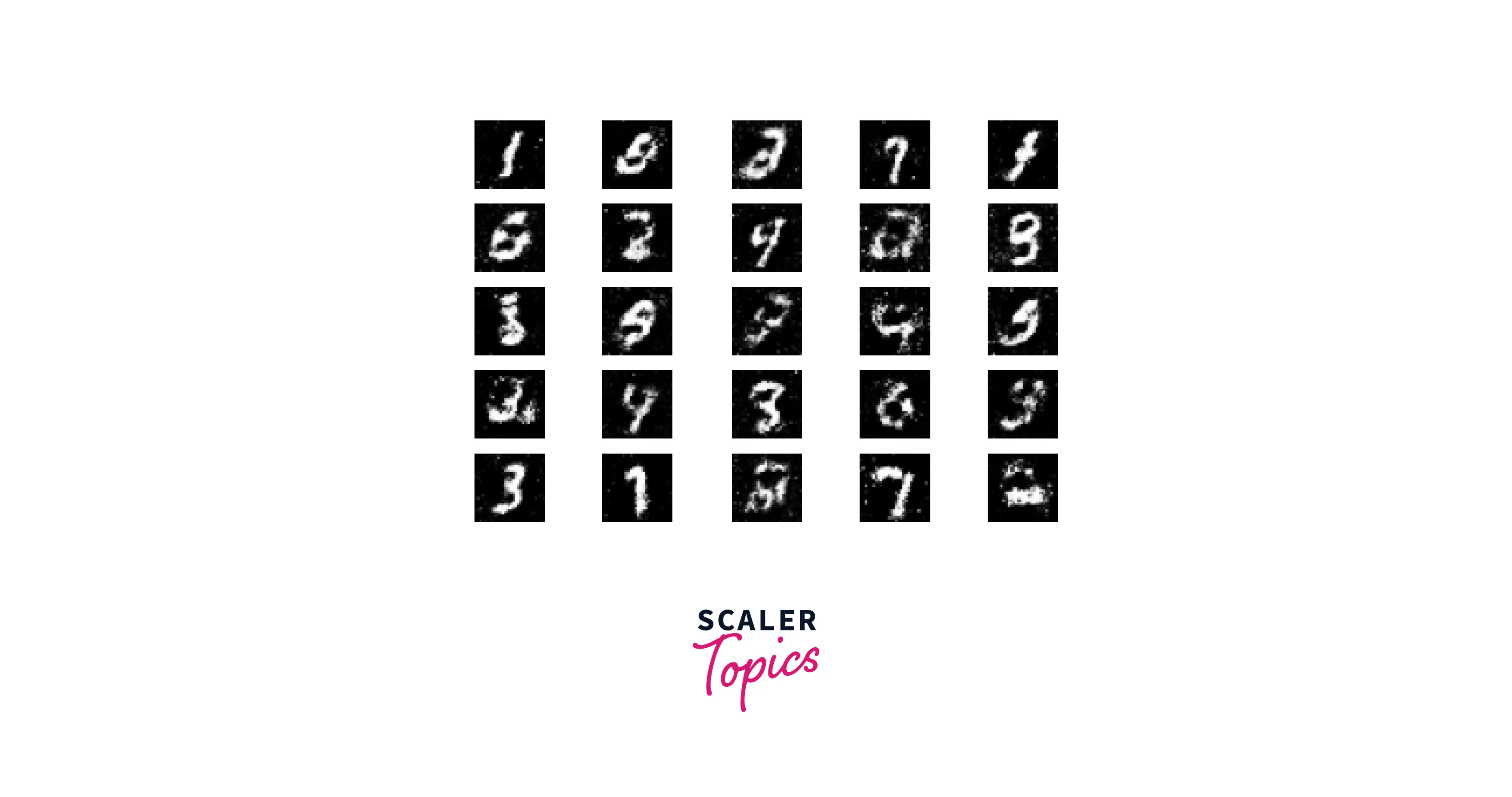
These images look very close to the handwritten number data we fed the network. Note that none of these exact images was previously shown to the network, and the network generated these as we trained it.