How to Hide or Unhide Columns and Rows in Excel?

How to Hide Columns in Excel?

Here are the steps for hiding columns in Excel:

• Click the first column, hold down the Shift key, and click the last column to select multiple neighboring columns.
• By clicking the first column while holding down the Control key (Command on a Mac), you can select numerous non-adjacent columns simultaneously.
• Use the name field:
  Enter a cell label in the name box to the left of the formula field. For instance, type B2 if you want to hide the second column. (For further information, see our Excel name box guide.)
• Once you've chosen, use one of these techniques to make the columns invisible.
• To hide a selected column, pick Hide from the context menu by right-clicking. (If you have already written the column identification, this method won't work.)
• To hide multilple columns, use Ctrl + 0 on your keyboard.
• Choose the Home tab, then select Format > Hide and Unhide and hide Columns from the Cells group.

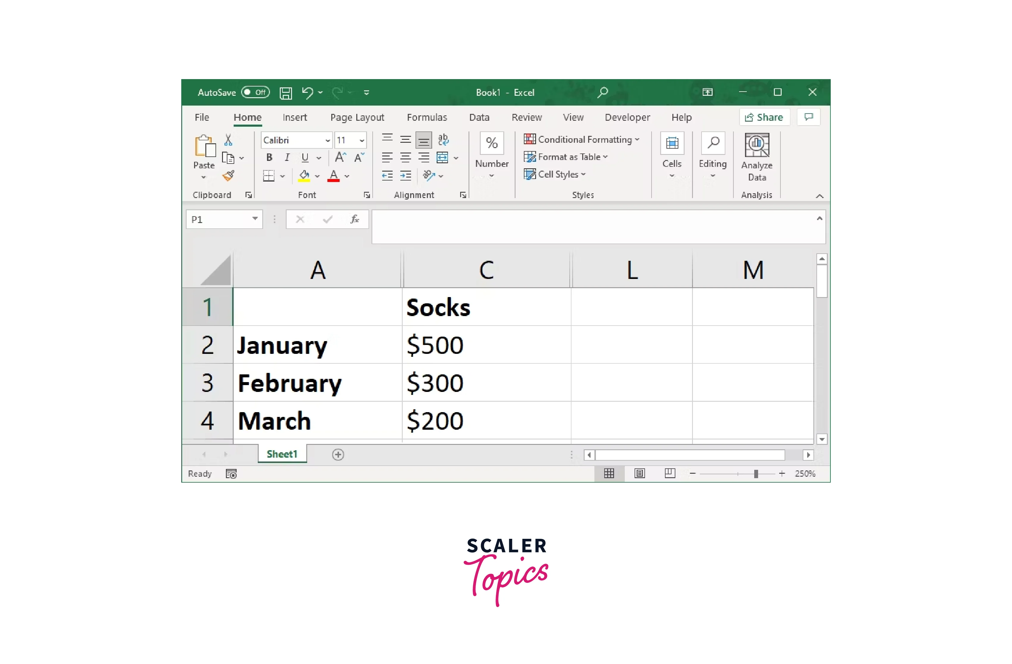
You'll notice a thin double line indicating the location of the hidden column or row in addition to the column or row being hidden.

How to Unhide Columns in Excel?

A few methods exist for how to unhide columns in Excel, choosing and displaying columns:

• Choose Unhide by right-clicking the slender double line that denotes a hidden row or column.
• Choose the two adjacent columns or rows. Choose Unhide Columns under Format > Hide and Unhide on the Home tab's Cells group.
• Use the keyboard shortcut Ctrl + A (Command + A on a Mac) to select all columns in your spreadsheet, then right-click and select Unhide.

Remember that while you can hide or unhide numerous columns simultaneously, you cannot unhide or hide both columns simultaneously.

How to Hide Rows in Excel?

Choose the row or rows that you want to hide first. This can be accomplished in several ways.

• Choose several adjacent rows:
  Press the first row while holding down the Shift key, then press the last row.
• Choose several distant rows:
  Click the first row, then click each next row while holding down the Control (Command on a Mac) key.
• Use the name field:
  In the name box to the left of the formula field, enter a cell label. For instance, type B2 if you wish to hide the second row. (For further information, see our Excel name box guide.)

Once you've chosen, use one of these techniques to hide the rows.

• To hide a chosen row, pick Hide from the context menu by right-clicking. (If you have already inputted the column or row identification, this method won't work.)
• Ctrl + 9 can be used to quickly hide rows.
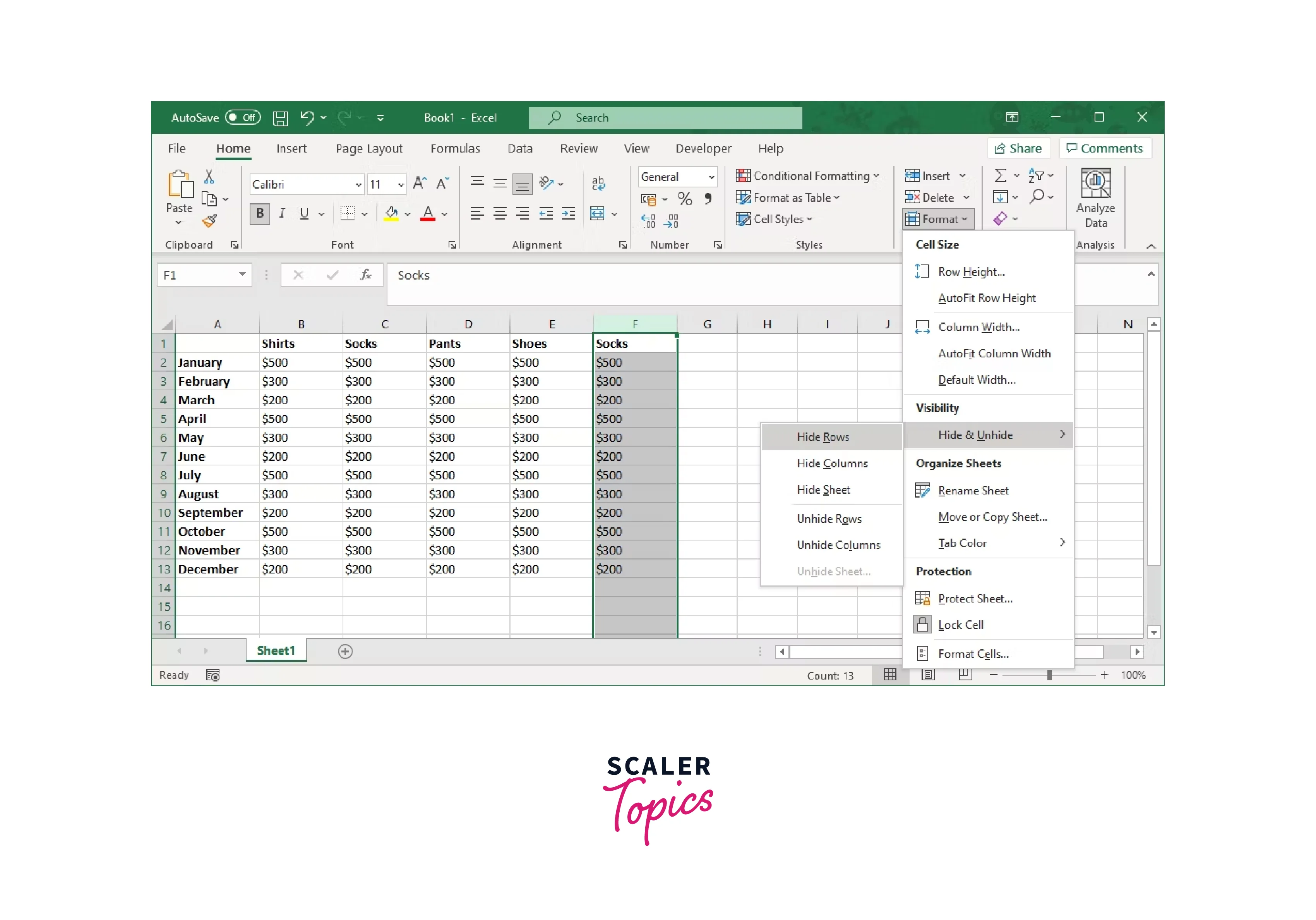
• Choose the Home tab, then select Format > Hide and Unhide and Hide Rows from the Cells group.

Summary:

• Choose the row you want to hide or one of its cells.
• Click Format under the Cells heading on the Home tab.
• Simply select Hidden & Unhide from the Format submenu.
• Choose Hide Rows.

How to Unhide Rows in Excel?

Many techniques exist for choosing and unhiding the rows:

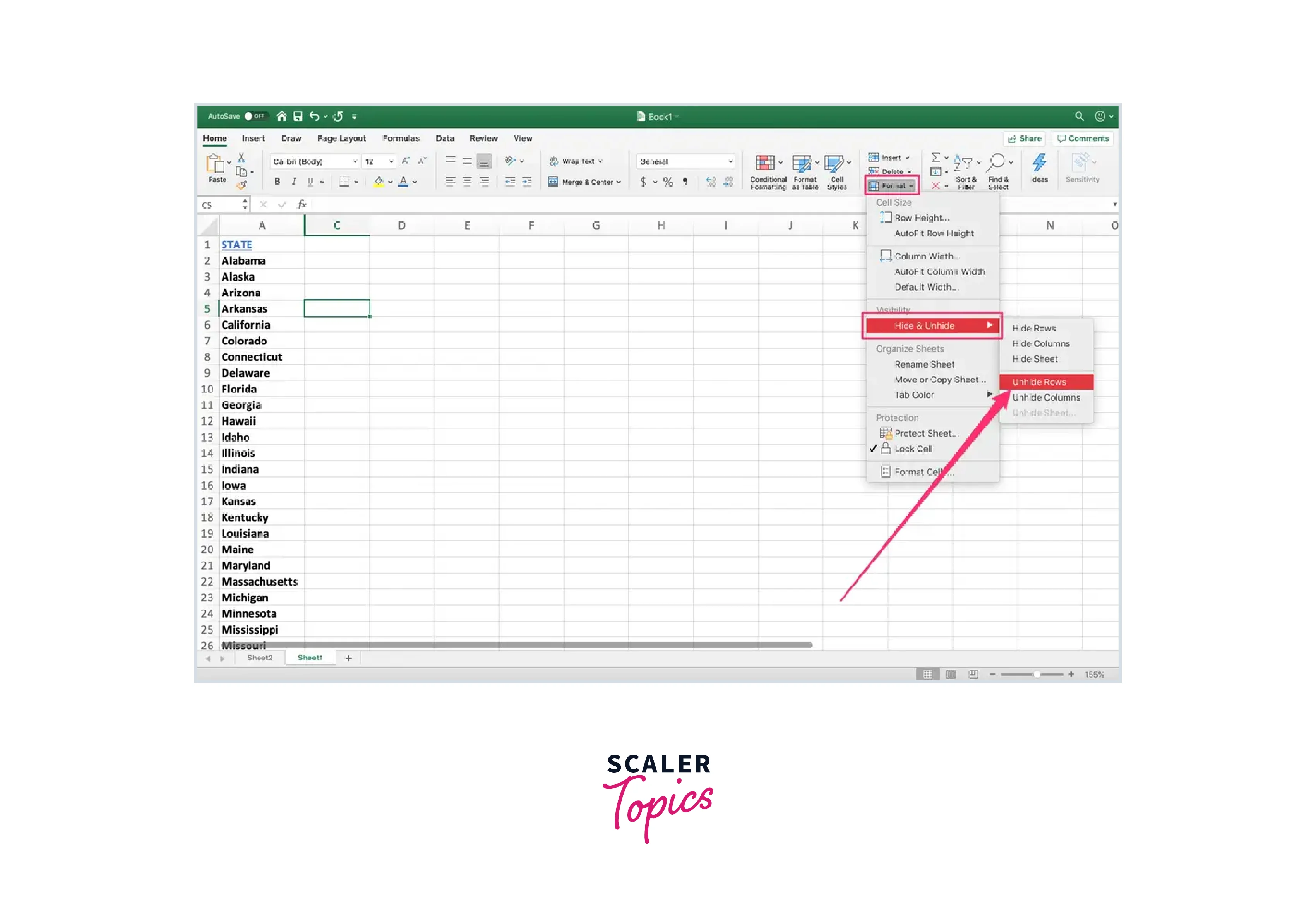
• To unhide a hidden row, right-click the thin double line and choose Unhide.
• Choose the two adjacent columns or rows. Choose Unhide Rows under Format > Hide and Unhide on the Home tab's Cells group.
• Use the keyboard shortcut Ctrl + A (Command + A on a Mac) to select all rows in your spreadsheet, then right-click and select Unhide.

Hide More Than Rows and Columns in Excel

In Excel, hiding rows and columns is a common practice when you want to temporarily remove unnecessary data from view. However, Excel's capabilities go beyond just hiding rows and columns. Here are a few other elements that you can hide in Excel:

1. Worksheets:
   You can hide entire worksheets in Excel by right-clicking on the worksheet tab you want to hide and selecting "Hide". To unhide, right-click on any worksheet tab and select "Unhide". A dialog box will pop up with a list of hidden worksheets. Select the one you want to unhide and click "OK".
2. Formulas:
   Excel allows you to hide formulas in two steps: first, select the cells with formulas you want to hide, right-click and select "Format Cells", then under the "Protection" tab, check "Hidden". Second, go to the "Review" tab and select "Protect Sheet". Now, anyone using the sheet cannot see or select the formulas in the cells you've chosen.
3. Gridlines:
   To hide gridlines, go to the "View" tab in the ribbon, and in the "Show" group, uncheck "Gridlines".
4. Cells:
   You can hide specific cells by making the text color the same as the cell background color. This is not technically hiding but makes the content invisible unless the cell is selected.
5. Data in Charts:
   In Excel, you can hide data in charts without deleting or hiding the entire row or column. Select the chart, go to the "Design" tab, and click "Select Data". In the "Select Data Source" dialog box that opens, you can remove series or categories from the chart.
6. Zero Values:
   To hide zero values, go to the "File" tab and select "Options". In the Excel Options dialog box, select "Advanced". Under "Display options for this worksheet", uncheck "Show a zero in cells with zero value".
7. Comments and Notes:
   To hide comments and notes, go to the "Review" tab, and click "Show All Comments". Clicking it once will show all comments, and clicking it again will hide them.

Remember, hiding data doesn't remove it from the spreadsheet, and can still be included in calculations. Always be aware of what data is hidden when interpreting Excel calculations.