Implementing DCGAN to generate CIFAR images

What are We Building?

One of the strengths of Generative Adversarial Networks (GANs) is the ability to create novel images. In this article, a DCGAN for image generation will be constructed using the CIFAR dataset. The DCGAN is a type of GAN that builds upon the Vanilla GAN and addresses some of its issues. The DCGAN is a good choice if the image data size exceeds $28x28$. This network also leads to fewer chances of a mode collapse and is thus a better network than a standard GAN. Here, we want the network to create realistic images to resemble any of the ten classes of the CIFAR dataset. We will create the DCGAN from scratch using PyTorch, train it, and write scripts to generate our images.

Pre-Requisites

Some prerequisites to understanding this article better:

• Basic understanding of Deep Learning and Neural Networks.
• Knowledge of Python programming language.
• Familiarity with TensorFlow or a similar deep learning framework.
• Understanding of Generative adversarial networks and their concepts.
• Knowledge of image processing and computer vision techniques.
• Familiarity with Convolutional Neural Networks (CNNs).
• Understanding of the CIFAR dataset and its structure.

What are DCGANs?

Researchers created the Vanilla GAN architecture to generate images in an unsupervised manner from image datasets. But this GAN had quite a few flaws that impacted its training. DCGANs are a modification of the Vanilla GAN architecture. The implementation of the Discriminator and Generator is configured to tackle some of the issues of the original GAN. Some of the changes are as follows. Convolutional layers are used explicitly in the Discriminator. In this architecture, the Generator explicitly uses Transposed Convolution layers. The Discriminator relies on Batch Normalization along with LeakyReLU activations. The Generator, on the other hand, uses ReLU activations. The DCGAN image generation process is similar to the Vanilla GAN except for a few tweaks to the optimizer and the architecture.

How are We Going to Build this?

To build the DCGAN, we will use the Python library PyTorch. We will first import PyTorch and other required libraries. We then load the image dataset using a DataLoader, the CIFAR10 dataset. After we load the data, we create the functions that make up the DCGAN. We can then train the network on this dataset and generate new photorealistic images that look like they were part of the CIFAR10 dataset.

The below sections focus on implementing all the functions required to create a DCGAN image generation pipeline.

Final Output

The final output generated by the DCGAN is a set of photorealistic images that closely resemble images from the CIFAR10 dataset. The process of training the model allows the Generator to learn the underlying patterns and structures of the dataset, resulting in images that are highly similar to real images from the dataset. We can use the generated images for tasks such as image synthesis, data augmentation, and even creating new images for a dataset. The results of the image generation process can be visually inspected, with examples of the generated images shown below.

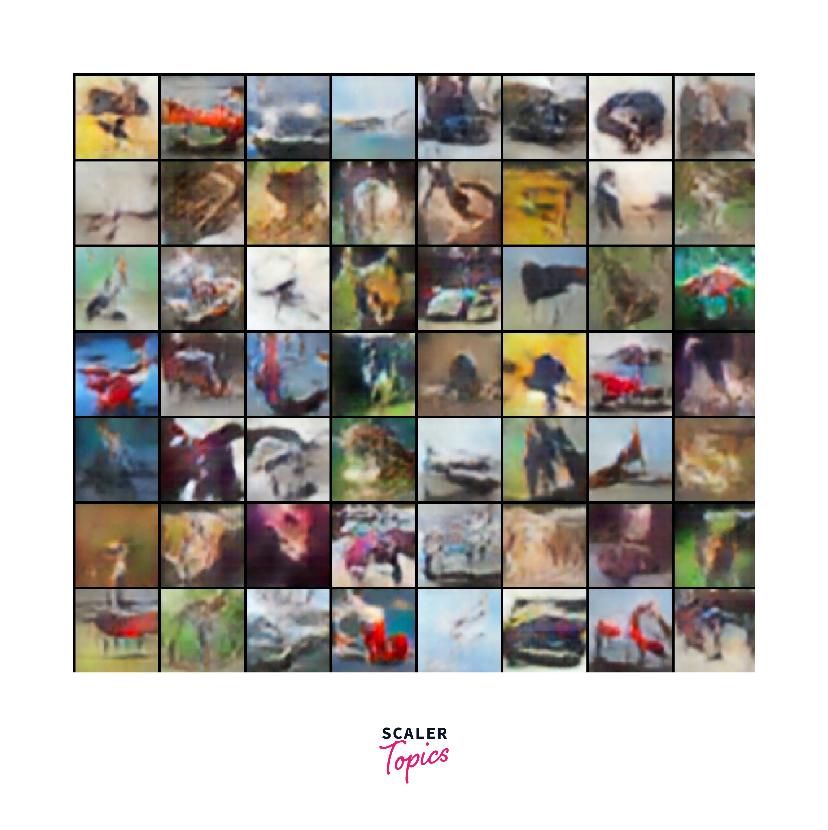
Note that longer training might yield better results but take significantly longer.

Requirements

• Before starting the DCGAN image generation process, we must import some libraries and perform set-up operations.
• First, we must create folders to store the models' images and weights using the mkdir command.
• We import the PyTorch library and all the required features we need that comes with it. We also import the numerical processing library numpy and the plotting library matplotlib.
• Training a GAN takes quite a long time. To further improve performance, we enable a flag in Pytorch that enables benchmarking. Pytorch runs a few checks on your current device during benchmarking to determine which algorithms perform best. These checks let you run slightly more optimized code for your current device.

Implementing DCGAN to Generate CIFAR Images

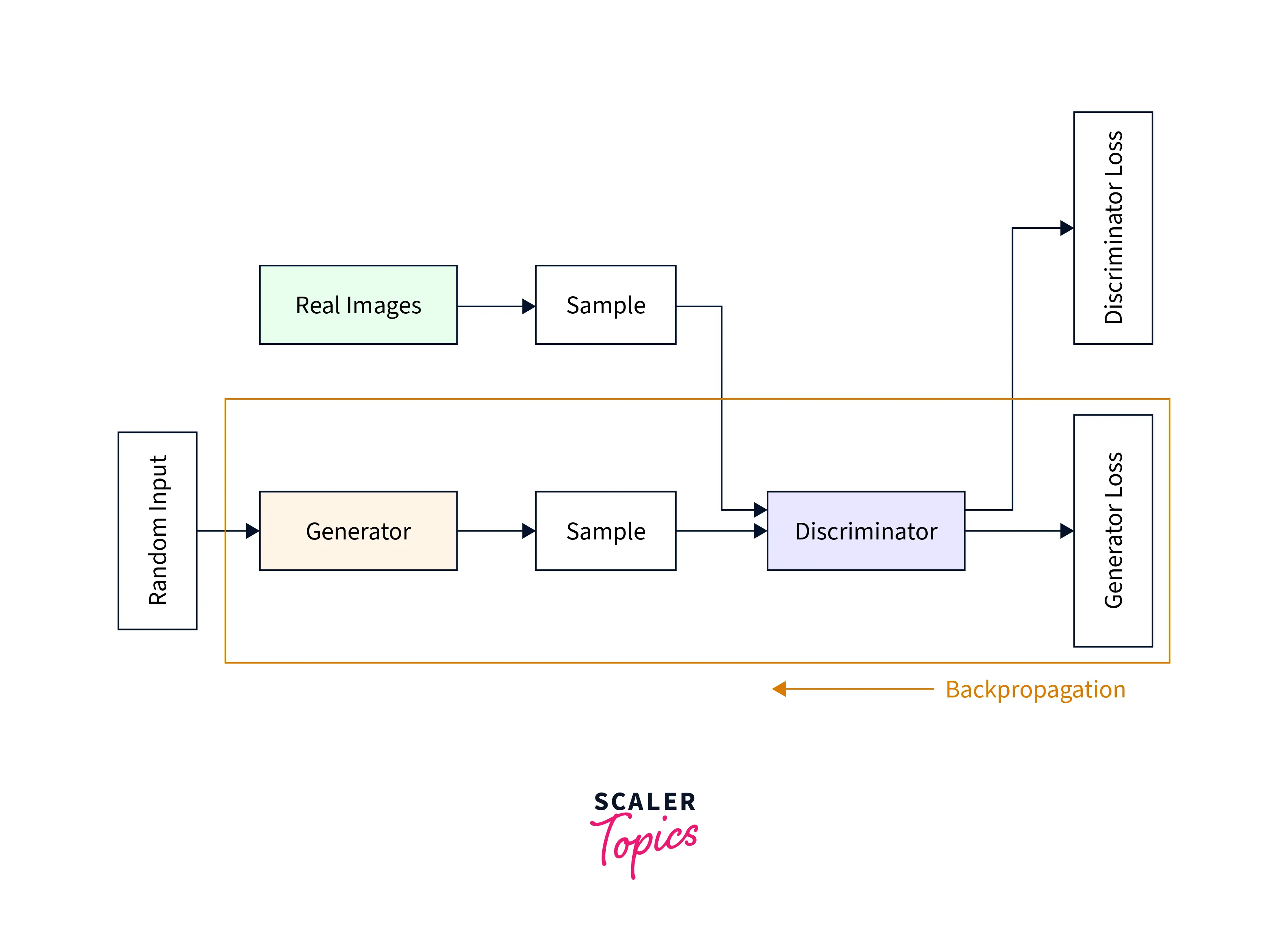
The main DCGAN image generation process involves creating a DataLoader, loading and preprocessing the CIFAR images, and sending batches of data to the GPU memory. The network architecture is then created, initialized, and sent to the GPU memory. After these initial steps, the network is trained to generate new images. The DCGAN architecture, like other GAN architectures, consists of a Generator and a Discriminator. The Generator creates photo-realistic images from random noise to fool the Discriminator. At the same time, the Discriminator takes the outputs of the Generator and returns the probability that the generated image is real. The Generator uses this probability to improve its generation capabilities by training the model.

The architecture diagram of the DCGAN is shown below.

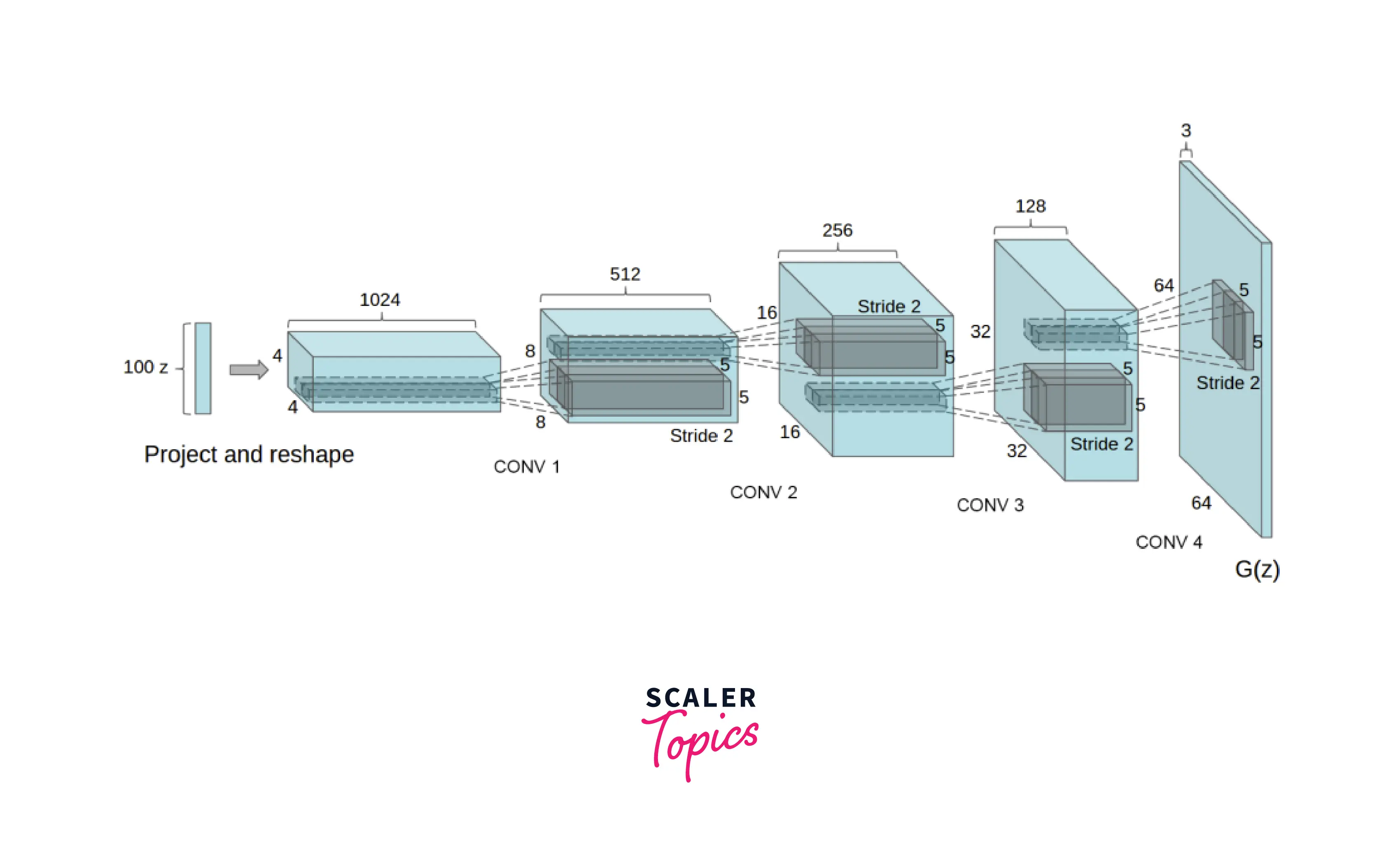
• GPU: the number of GPUs. In this case, we will only be using a single one.
• nz: the width of the input.
• ngf and ndf denote the shape of the maps that the Generator and Discriminator create, respectively.
• nc is the number of channels that the image has.

We first start by loading our data and understanding how it looks.

Exploring the Dataset

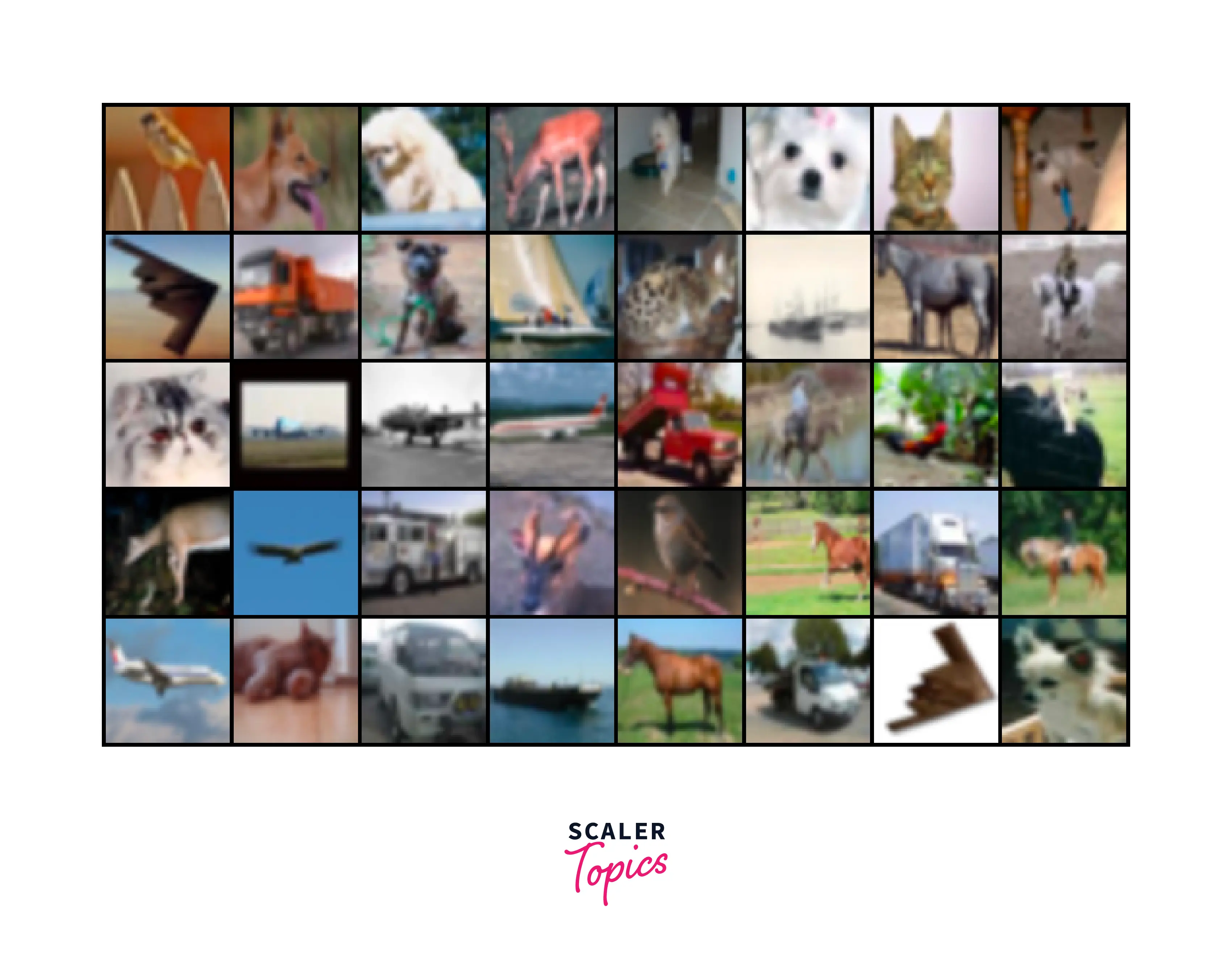
This article will use the CIFAR10 (Canadian Institute for Advanced Research) dataset to build a DCGAN for image generation. The CIFAR10 dataset contains ten classes of images in a 3-channel RGB format, similar to the MNIST format. It's a common dataset for benchmarking image classification models, and it's easy for a model to learn. To use the dataset, we first load and preprocess it.

PyTorch has the CIFAR10 dataset inbuilt, and we can directly load it. However, if it's the first time we're using it, we must download it first. After that, we resize all the images to a common size of $64x64x3$. Although CIFAR10 is a clean dataset, this resizing step is a good practice. We also normalize the images and convert them to PyTorch tensors. In PyTorch, we create a DataLoader, a class that creates optimized batches of data to pass to the model. To enhance the speed of the DCGAN image generation process, we send the DataLoader to the GPU if we're using one.

After loading the data, we can see how it looks. To visualize a batch of data, we iterate over the DataLoader to grab a single batch of images. After obtaining the images, we can create a grid the size of a single batch, pad the images to make them look neater, and normalize them. This batch of images is still on the GPU, so we cannot plot it on the CPU without sending it back.

As we can see, the dataset comprises ten classes of images from which we plot a random sample.

Defining the Discriminator

The Discriminator in the DCGAN is responsible for classifying the images returned by the Generator as real or fake. Architecturally, the Discriminator is almost a mirror of the Generator with minor differences. The Discriminator uses a Strided Convolution and a LeakyReLU along with Batch Normalization layers. The final layer is a Sigmoid layer that returns the probability we want. For DCGAN image generation, the Discriminator uses Strided Convolutions instead of Pooling layers. This choice allows the network to learn custom padding functions that, in turn, improve performance.

Defining the Generator

The Generator is responsible for mapping the input data from the latent to the vector data space. In this part of the network, we get an RGB image as an output that can then be passed to the Discriminator. The generated image size is identical to the original training images but in channel first indexing ($3x64x64$). The Generator comprises blocks with Transposed Convolutions, Batch Normalizations, and ReLU layers. The final layer has a Tanh activation used to make the data to a range of [-1,1]. In this part of the DCGAN image generation process, the DCGAN uses Batch Normalization layers after Transposed convolutions. This shift enables a smoother gradient flow between the layers of the network.

Defining the Inputs

We need to set up some empty containers for an optimized workflow. We first create a fixed noise with the shape (128, size of latent space, 1, 1) and send it to the GPU. We also denote the label of the real image as one and the fake image as 0. For this article, we will run the network for 25 epochs.

We also pre-allocate arrays to store the Generator and Discriminator loss during training.

Computing the Loss Function

The DCGAN image generation pipeline has two loss functions, for the Generator and Discriminator, respectively. The Discriminator penalizes wrongly classifying a real image as a fake or a fake image as real. This concept can be thought of as maximizing the following function.

$\nabla_{\theta_{d}} \frac{1}{m} \Sigma_{i=1}^{m}[log D(x^{(i)}) + log(1-D(G(z^{(i)})))]$

The Generator loss takes the output of the Discriminator into account and rewards it if the Generator is fooled into thinking the fake image is real. If this condition is not satisfied, the Generator is penalized. This concept can be thought of as minimizing the following function.

$\nabla_{\theta_{g}} \frac{1}{m} \Sigma_{i=1}^{m}log(1-D(G(z^{(i)})))$

Optimizing the Loss

We will use the ADAM optimizer with a learning rate of 0.0002 and the beta parameters set to (0.5, 0.999) to optimize the loss. The Generator and Discriminator have different optimizers to ensure they both learn independently.

Train the DCGAN

To run DCGAN image generation, we need to train the network first. The general procedure is as follows. For each epoch, the noise is sent to the Generator. The Discriminator also gets a random image sampled from the dataset. The Generator then uses the weights it has learned to modify the noise to be closer to the target image. In doing so, the Generator learns a mapping between random noise and the latent space of the image dataset. The Generator then sends the tweaked image to the Discriminator. The Discriminator then predicts how real it thinks the generated image is and informs the Generator using a probability metric.

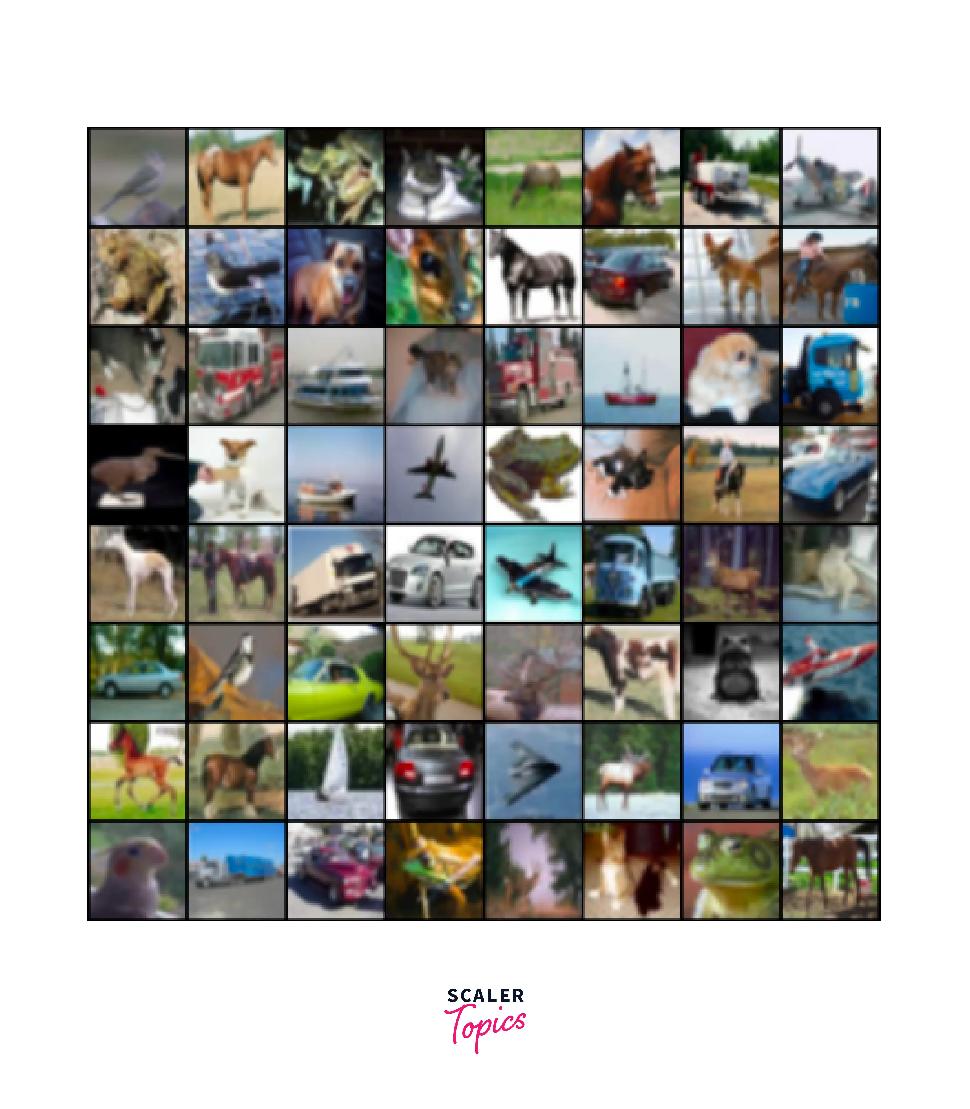
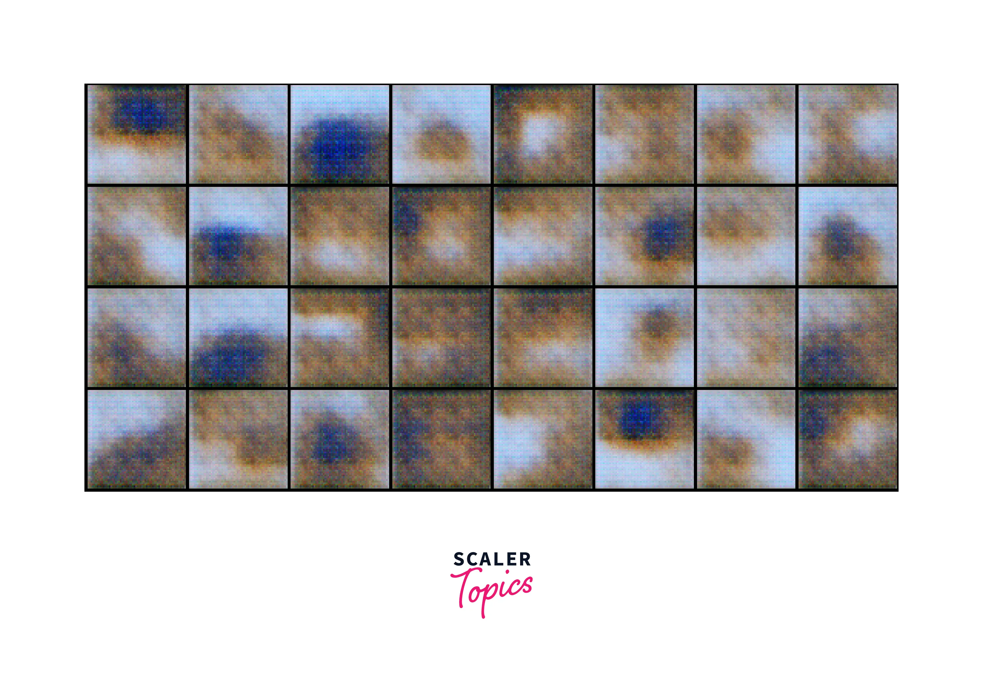
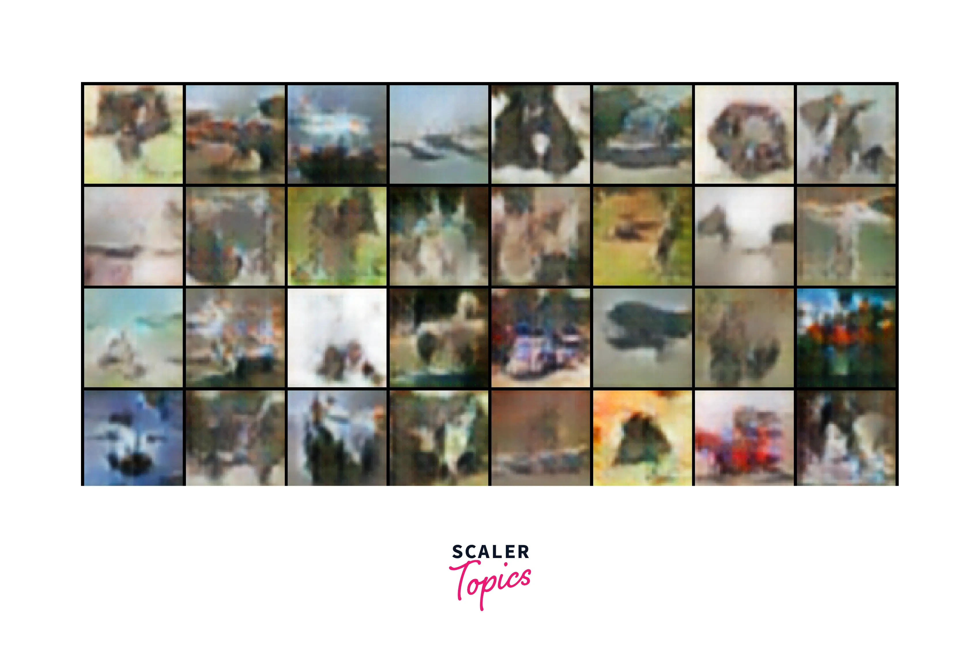
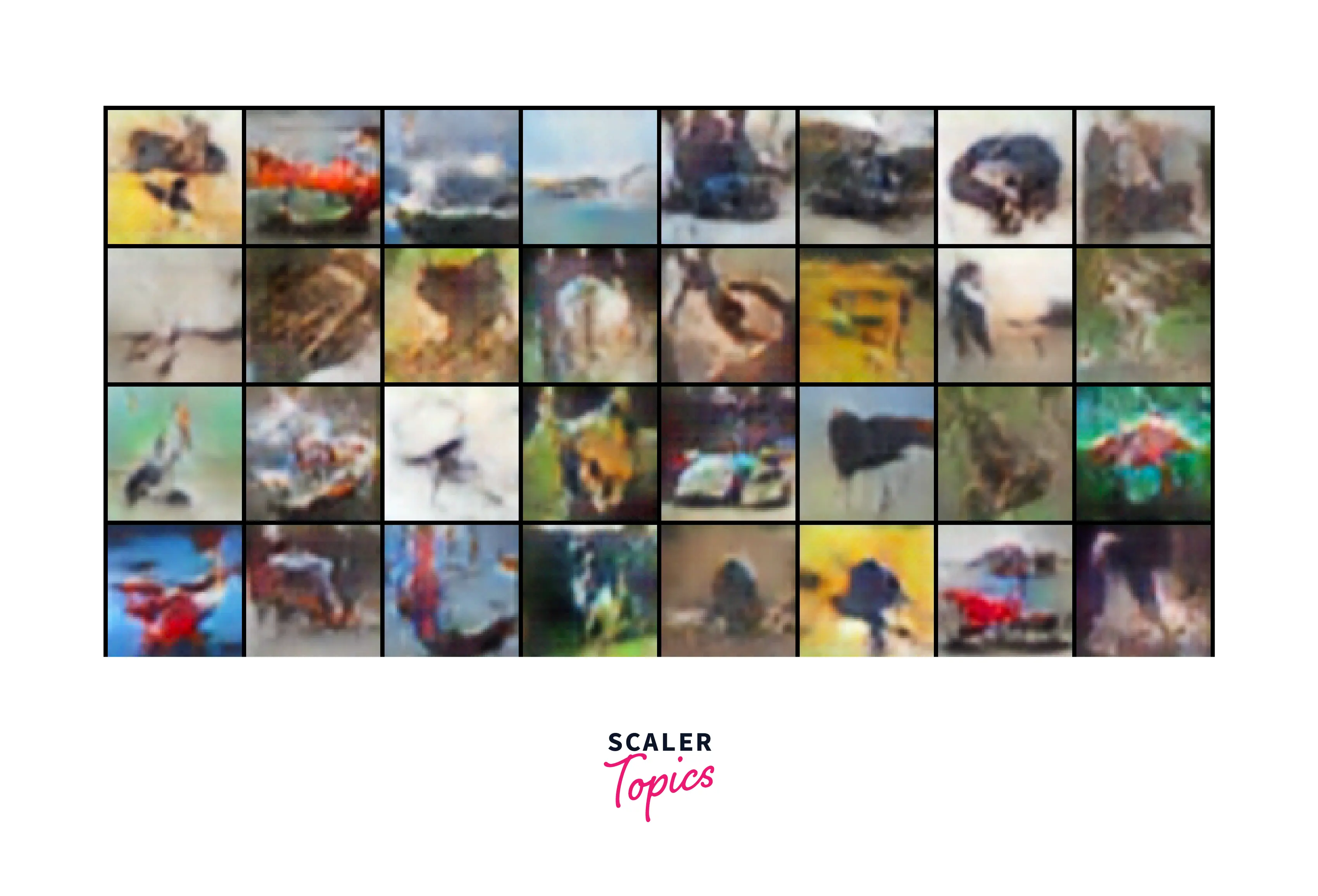
In this article, we train the network for 25 epochs. After the training is complete and even during training, we can periodically check the ./images folder to see outputs for every 100 steps. The results we get are as follows.

We look at the original sample and the outputs at 0, ten, and 25 epochs to understand the training progression.

What's Next

We can apply a few tweaks to the DCGAN in further experiments. Some of them are mentioned below.

• Tweaking the z_size variable and either increasing or decreasing it might lead to better performance.
• Longer training might also lead to better results.
• Using Label Smoothing Cross Entropy Loss instead of just a Cross Entropy Loss might also improve performance.
• There is a long list of tweaks proposed by one of the creators of the PyTorch library regarding the DCGAN. The article mentioned is quite a few years old but gives a good background for further DCGAN image-generation process experiments.