Kalman Filter in Computer Vision
Overview
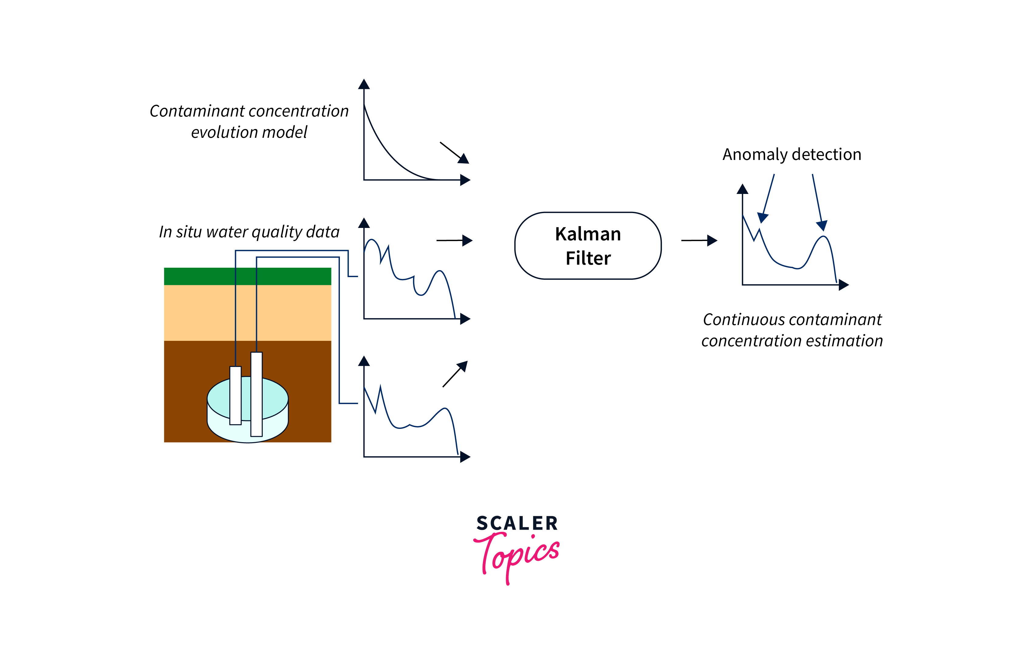
Kalman filter in computer vision is a mathematical algorithm that is widely used for signal processing, control systems, and particularly for estimation problems in robotics and computer vision. In computer vision, the Kalman filter is used for tracking, image filtering, and object recognition. In this article, we will focus on the key aspects and theory of the Kalman filter, its advantages, and limitations.
What is Image Classification?
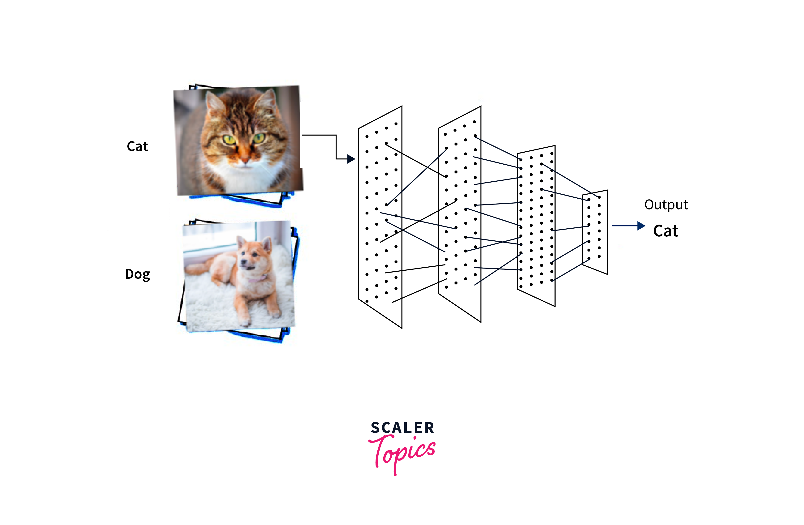
Image Classification is a process of assigning a label or a category to an image based on its content. It is one of the fundamental problems in computer vision and machine learning. The goal of image classification is to teach a computer to recognize objects in an image and classify them into predefined categories. For example, given an image of a dog, the classifier should label it as a "dog" and not as a "cat" or any other object.
What is Kalman Filter?
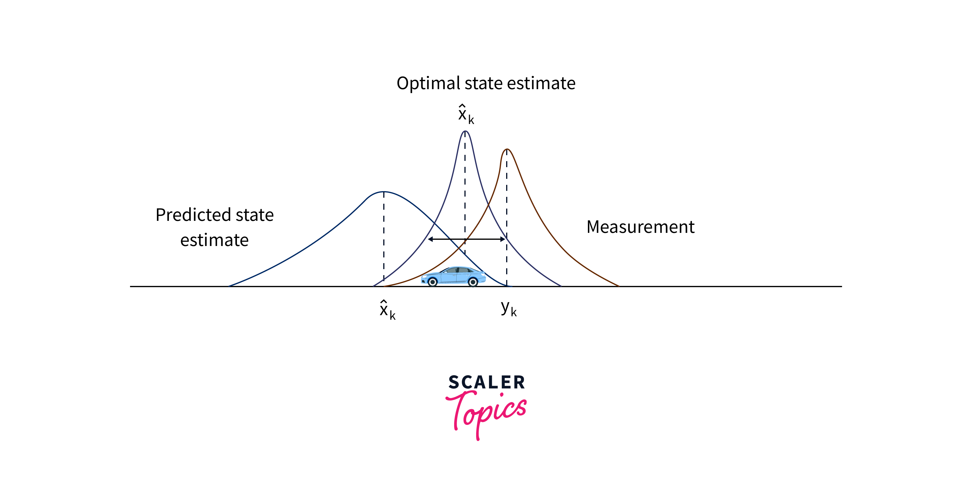
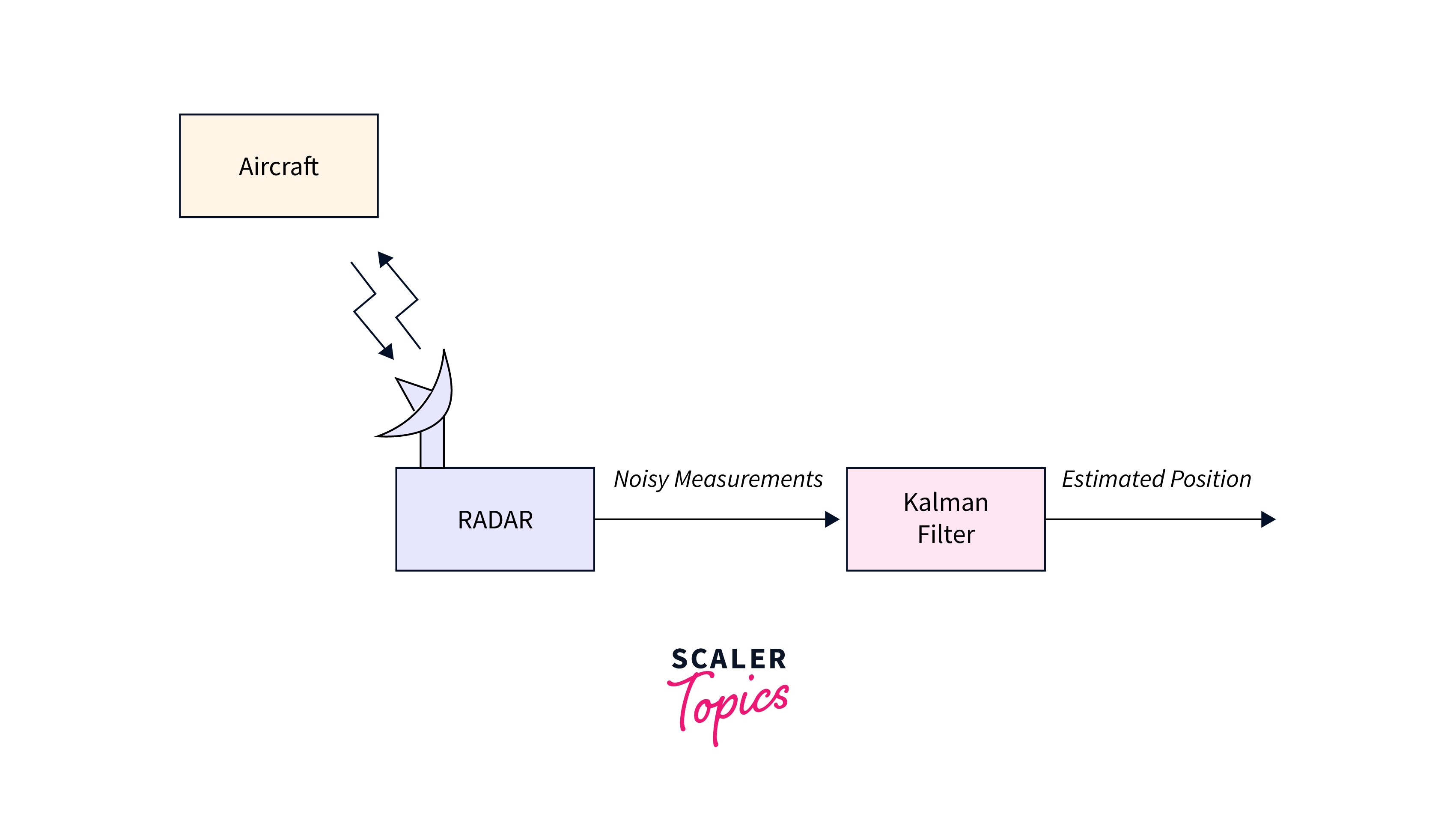
The Kalman filter is a mathematical algorithm that estimates the state of a system by combining noisy measurements with a prediction of the system's state based on a mathematical model. It was first developed by Rudolf Kalman in 1960 for spacecraft navigation. The Kalman filter in computer vision is widely used in various applications such as signal processing, control systems, and particularly for estimation problems in robotics and computer vision.
- The Kalman Filter in computer vision is based on the principles of Bayesian estimation, where it uses a probabilistic approach to update the system's state estimate based on prior knowledge and new measurements.
- The Kalman Filter provides an optimal estimate of the system's state by minimizing the mean square error between the estimated state and the true state, considering both the predicted state and the measurements.
- The filter predicts the future state of the system based on the current state estimate and the known dynamics of the system, utilizing a linear mathematical model.
- The Kalman Filter in computer vision incorporates new measurements into the state estimation process, adjusting the predicted state based on the observed values and their associated uncertainties.
Key Aspects of Kalman Filter
The Kalman filter in computer vision has several key aspects that make it popular for estimation problems in robotics and computer vision. These aspects include:
-
State Space Model: The Kalman filter models the system as a set of mathematical equations that describe the system's state, the measurements, and the noise in the system.
-
Prediction Step: The Kalman filter in computer vision predicts the future state of the system based on the previous state and the system's mathematical model.
-
Correction Step: The Kalman filter corrects the predicted state using the measurements obtained from the system.
Step Formula State Space Model State Equation x(k) = Ax(k-1) + Bu(k) + w(k) Measurement Equation z(k) = Hx(k) + v(k) Prediction Step State Prediction Error Covariance Prediction Correction Step Kalman Gain State Correction Error Covariance Correction
Theory of Kalman Filter
The Kalman filter is based on the theory of Bayesian statistics. It estimates the state of a system by combining a prediction of the state based on a mathematical model with the measurements obtained from the system. The Kalman filter assumes that the noise in the system follows a normal distribution, and the measurements are independent and identically distributed.
The Kalman Filter utilizes the Bayesian update rule to compute the posterior probability of the system state given the measurements. It combines the prior belief (predicted state) and the likelihood (measurement) to obtain the posterior belief (updated state estimate).
State space model
The Kalman filter in computer vision models the system as a set of mathematical equations that describe the system's state, the measurements, and the noise in the system. The state of the system is represented by a vector, and the measurements are represented by another vector. The mathematical model of the system is represented by a set of matrices.
The Kalman Filter assumes that the system dynamics can be modeled using linear equations with additive Gaussian noise. The state transition and measurement equations are typically represented as follows:
State Transition Equation: KaTeX parse error: Expected 'EOF', got 'ₖ' at position 2: xₖ̲ = Fₖ₋₁xₖ₋₁ + B…
Measurement Equation: KaTeX parse error: Expected 'EOF', got 'ₖ' at position 2: zₖ̲ = Hₖxₖ + vₖ
where,
- KaTeX parse error: Expected 'EOF', got 'ₖ' at position 2: xₖ̲ is the system state at time step k
- KaTeX parse error: Expected 'EOF', got 'ₖ' at position 2: Fₖ̲₋₁ is the state transition matrix from time step k-1 to k
- KaTeX parse error: Expected 'EOF', got 'ₖ' at position 2: Bₖ̲₋₁ is the control input matrix
- KaTeX parse error: Expected 'EOF', got 'ₖ' at position 2: uₖ̲₋₁ is the control input vector
- KaTeX parse error: Expected 'EOF', got 'ₖ' at position 2: wₖ̲₋₁ is the process noise (assumed to be Gaussian with mean zero and covariance Qₖ₋₁)
- KaTeX parse error: Expected 'EOF', got 'ₖ' at position 2: zₖ̲ is the measurement at time step k
- KaTeX parse error: Expected 'EOF', got 'ₖ' at position 2: Hₖ̲ is the measurement matrix
- KaTeX parse error: Expected 'EOF', got 'ₖ' at position 2: vₖ̲ is the measurement noise (assumed to be Gaussian with mean zero and covariance Rₖ)
Prediction step
The Kalman filter predicts the future state of the system based on the previous state and the system's mathematical model. The prediction is made by multiplying the previous state by the system's matrix and adding the noise in the system.
In the prediction step, the Kalman Filter estimates the predicted state KaTeX parse error: Expected 'EOF', got 'ₖ' at position 3: x̂ₖ̲₋₁|ₖ₋₁ and the predicted error covariance Pₖ₋₁|ₖ₋₁ based on the previous state estimate and the system dynamics. The formulas for the prediction step are as follows:
Predicted State: KaTeX parse error: Expected 'EOF', got 'ₖ' at position 3: x̂ₖ̲₋₁|ₖ₋₁ = Fₖ₋₁x̂…
Predicted Error Covariance: KaTeX parse error: Expected 'EOF', got 'ₖ' at position 2: Pₖ̲₋₁|ₖ₋₁ = Fₖ₋₁Pₖ…
Correction step
The Kalman filter in computer vision corrects the predicted state using the measurements obtained from the system. The correction is made by comparing the predicted state with the measurements and adjusting the predicted state based on the difference between them.
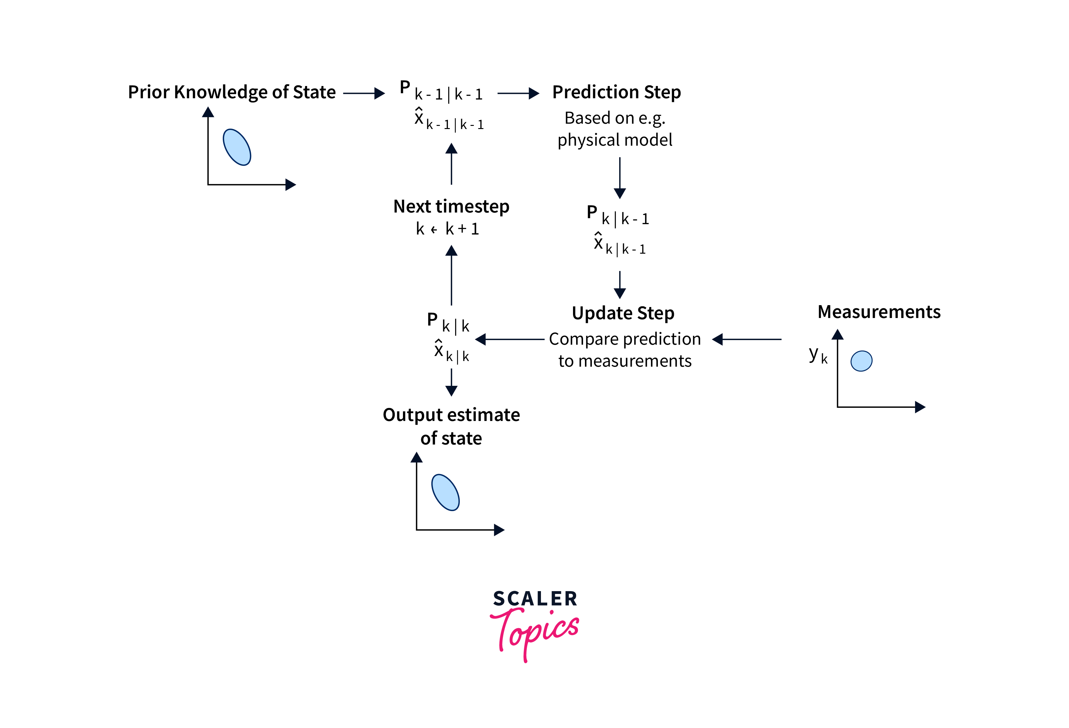
In the update step, the Kalman Filter combines the predicted state with the actual measurement to obtain an updated state estimate KaTeX parse error: Expected 'EOF', got 'ₖ' at position 3: x̂ₖ̲|ₖ and an updated error covariance KaTeX parse error: Expected 'EOF', got 'ₖ' at position 2: Pₖ̲|ₖ. The formulas for the update step are as follows:
Kalman Gain: KaTeX parse error: Expected 'EOF', got 'ₖ' at position 2: Kₖ̲ = Pₖ₋₁|ₖ₋₁Hₖᵀ(…
Updated State Estimate: KaTeX parse error: Expected 'EOF', got 'ₖ' at position 3: x̂ₖ̲|ₖ = x̂ₖ₋₁|ₖ₋₁ …
Updated Error Covariance: KaTeX parse error: Expected 'EOF', got 'ₖ' at position 2: Pₖ̲|ₖ = (I - KₖHₖ)…
By recursively applying the prediction and update steps, the Kalman Filter continuously refines its estimate of the system state, incorporating new measurements and adjusting for uncertainties. It optimally combines the predicted state with the measurements, balancing the information from both sources to provide an accurate and reliable estimate of the true state.
Advantages of Kalman Filter
The Kalman filter in computer vision has several advantages that make it popular for estimation problems in robotics and computer vision. These advantages include:
- Optimal Estimation: The Kalman Filter achieves optimal estimation by considering both the predicted state and the measurements. It takes into account the uncertainties associated with the predictions and measurements, weighting them appropriately in the estimation process. By minimizing the mean square error between the estimated state and the true state, the Kalman Filter provides the best possible estimate given the available information. It achieves this optimality by iteratively updating the state estimate based on the Kalman gain, which balances the confidence in the prediction and the accuracy of the measurements. Through this optimization process, the Kalman Filter provides an accurate and robust estimation of the system's state.
-
Robustness: The Kalman Filter demonstrates robustness by effectively handling noise in the system. It accounts for the presence of noise in both the predicted state and the measurements, allowing it to filter out erroneous or misleading information. By incorporating the noise covariance matrices Q and R, the filter appropriately weighs the contributions of the predictions and measurements, reducing the impact of noisy measurements on the final state estimate. Additionally, the iterative nature of the Kalman Filter allows it to continuously update and refine the state estimate as new measurements are obtained, adapting to changing noise levels and improving robustness over time. This robustness makes the Kalman Filter suitable for applications in various domains where noisy measurements are common, such as sensor fusion, tracking, and control systems.
-
Real-Time Processing: The Kalman Filter is well-suited for real-time processing due to its computational efficiency and recursive nature. It updates the state estimate in a step-by-step manner as new measurements arrive, allowing for continuous and immediate estimation. This real-time processing capability enables the Kalman Filter to keep up with fast-changing systems and rapidly evolving environments, making it an ideal choice for time-sensitive applications such as navigation, robotics, and control systems.
Limitations of Kalman Filter
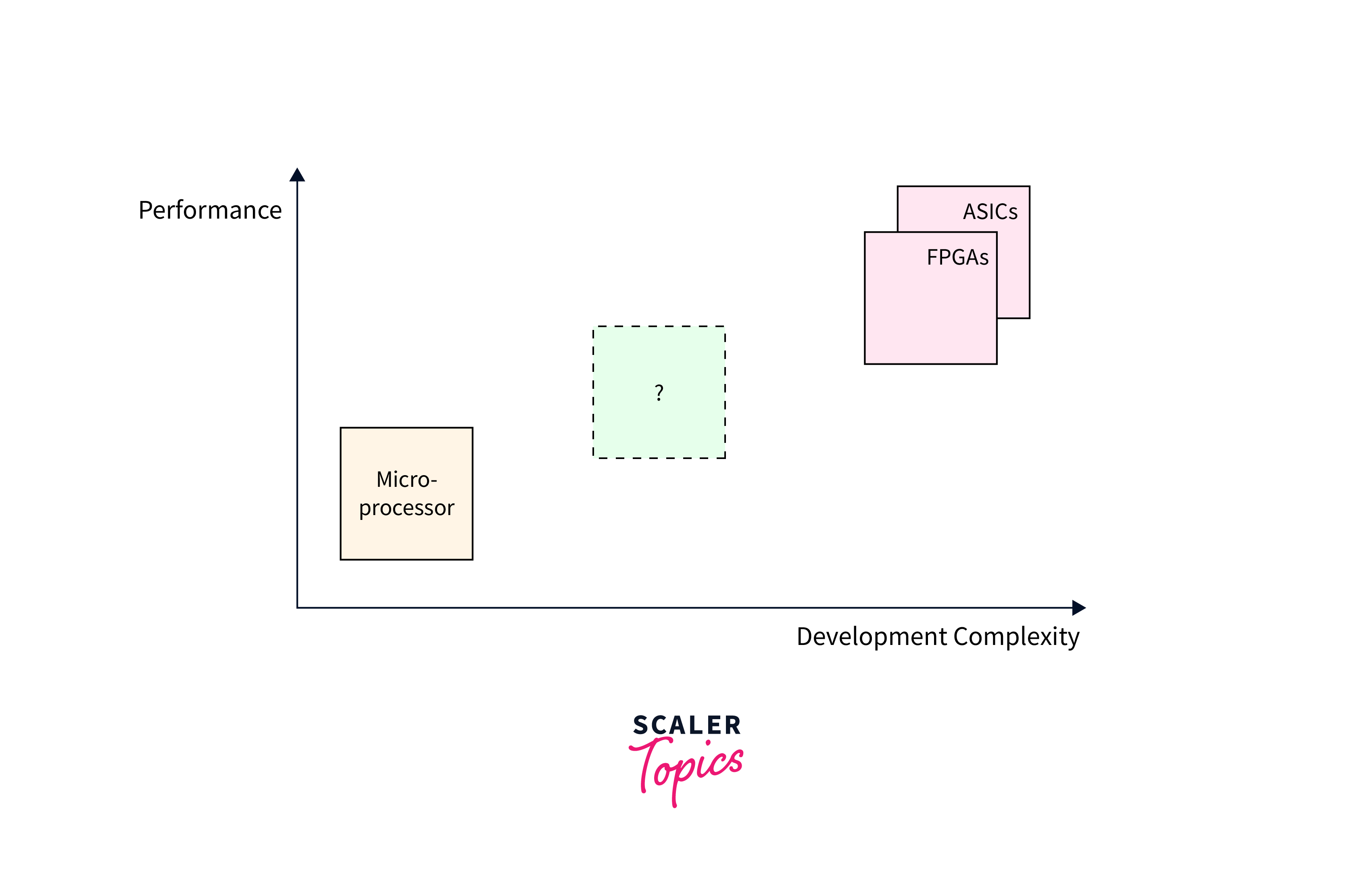
The Kalman filter in computer vision has several advantages such as robustness and real-time processing, but it also has limitations such as linearity, model uncertainty, and computational complexity that should be considered when using it for real-world applications. The pre-dominant limitations are listed below:
-
Linearity: The Kalman filter assumes that the system's mathematical model is linear, which limits its applicability to nonlinear systems. Nonlinear systems require more complex mathematical models and filtering algorithms.
-
Model Uncertainty: The Kalman filter assumes that the system's mathematical model is known and accurate, which may not be the case in real-world applications. Model uncertainty can lead to inaccurate estimates and affect the performance of the filter.
-
Computational Complexity: The Kalman filter in computer vision requires matrix operations that can be computationally intensive, especially for high-dimensional systems. This can limit the filter's applicability to real-time applications with limited computational resources.
OpenCV functions for Kalman Filter
These functions are part of the cv::KalmanFilter class in OpenCV and can be used to implement the Kalman filter for various applications in computer vision and robotics.
| Function | Description |
|---|---|
| cv::KalmanFilter::KalmanFilter(int dynamParams, int measureParams, int controlParams=0, int type=CV_32F) | Creates an instance of the Kalman filter class with the specified number of state, measurement, and control variables. |
| cv::KalmanFilter::init(cv::Mat state, cv::Mat cov, cv::Mat &mean) | Initializes the Kalman filter with the initial state and covariance matrix. |
| cv::KalmanFilter::predict(cv::Mat &control=cv::Mat()) | Predicts the state of the system based on the previous state and the system's mathematical model. |
| cv::KalmanFilter::correct(cv::Mat measurement) | Corrects the predicted state using the measurements obtained from the system. |
| cv::setIdentity(cv::Mat &mat, const cv::Scalar &s) | Sets the identity matrix for the specified matrix. |
| cv::randn(cv::Mat &mat, cv::Scalar mean, cv::Scalar stddev) | Generates a matrix of random numbers with a normal distribution. |
Implementation of Kalman Filter in Computer Vision
In computer vision, the Kalman Filter is commonly used for tracking and estimation tasks. It can be implemented to track objects in video sequences, estimate the position and motion of objects, and handle occlusions and noise. The filter's ability to handle uncertainties and update estimates in real-time makes it valuable for computer vision applications.
Let's have a detailed overview of the Python implementation of the Kalman filter in computer vision and understand each step in detail.
Step 1: Import Required Libraries We start by importing the necessary libraries for our implementation, which are OpenCV, NumPy, and Random.
Step 2: Define a Function to Plot the Estimated States
We define a function called plot_curve to plot the estimated states over time. The function takes two arguments x and y, which are NumPy arrays containing the x and y coordinates of the estimated states. The function uses OpenCV to draw a line between consecutive estimated states and displays the resulting plot.
The function first creates a black image using NumPy with a size of 600x800 pixels and 3 color channels. We then loop over the estimated states and draw a line between each consecutive pair of states. Finally, we display the resulting plot using OpenCV's imshow function and wait for a key press using waitKey.
Step 3: Define the Initial State Variables
We define two state variables state and state_pre, which are NumPy arrays with a size of 2x1 and a data type of float32. The state variable represents the current state of the system, while the state_pre variable represents the predicted state of the system.
Step 4: Define the State Transition Matrix
We define a 2x2 identity matrix as the state transition matrix A. This matrix describes how the system state evolves over time.
Step 5: Define the Measurement Matrix
We define a 1x2 matrix H as the measurement matrix. This matrix describes how the system state is related to the measurements.
In this example, we are measuring the x-coordinate of the system state. Therefore, we set the first element of the measurement matrix to 1 and the second element to 0.
Step 6: Define the Process Noise Covariance Matrix We define a 2x2 identity matrix multiplied by a small constant as the process noise covariance matrix Q. This matrix describes the uncertainty in the system dynamics.
In this example, we assume that the system dynamics are mostly deterministic, with some small amount of random noise added at each time step. Therefore, we set the process noise covariance matrix to a small constant multiplied by the identity matrix.
Step 7: Define the Measurement Noise Covariance Matrix
We define a scalar value R as the measurement noise covariance matrix. This matrix describes the uncertainty in the measurements.
In this example, we assume that the measurement noise is small and approximately Gaussian with zero mean and constant variance. Therefore, we set the measurement noise covariance matrix to a scalar value.
Step 8: Define the Kalman Filter
We define a Kalman filter object using OpenCV's KalmanFilter class. We set the size of the state to 2 and the size of the measurement to 1. We then set the state transition matrix, measurement matrix, process noise covariance matrix, and measurement noise covariance matrix using the set_* methods of the Kalman filter object.
Step 9: Generate Input Data
We generate a sequence of input data data containing 100 samples. We assume that the true state of the system follows a linear motion with a constant velocity of 10 units per second.
We assume that the measurements are corrupted by additive Gaussian noise with zero mean and a standard deviation of 1 unit.
Step 10: Apply the Kalman Filter in computer vision to the Input Data
We apply the Kalman filter to the input data using a for loop. At each time step, we predict the next state using the predict method of the Kalman filter object and update the state estimate using the current measurement and the correct method of the Kalman filter object. We also store the estimated states in the states NumPy array.
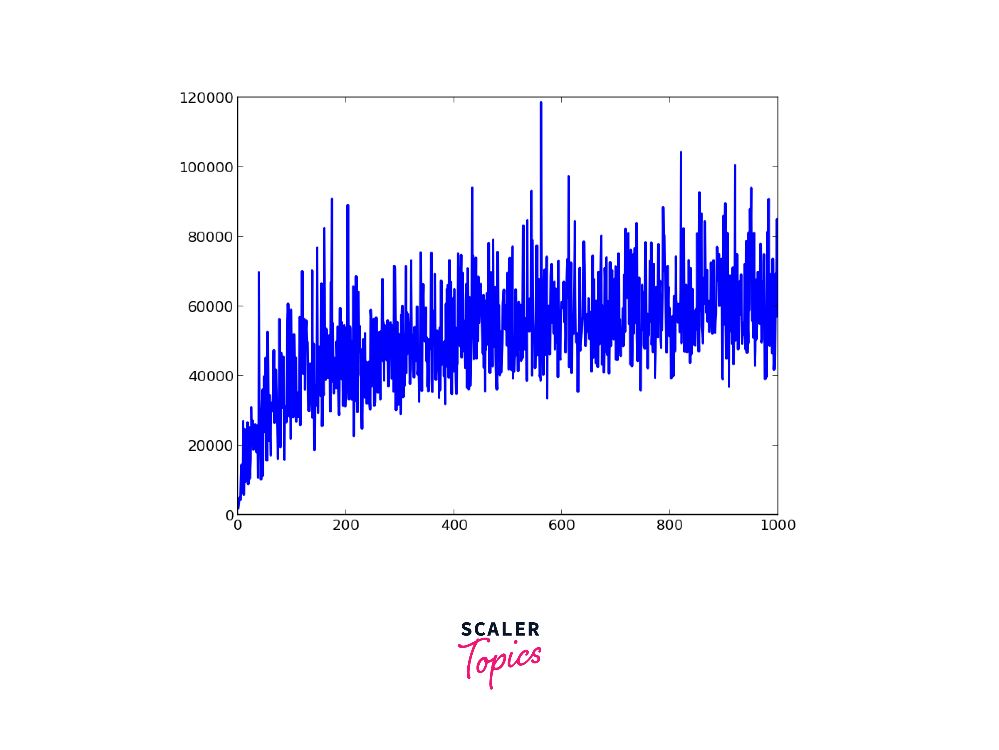
Step 11: Plot the Estimated States We plot the estimated states over time using the plot_curve function defined earlier.
Output
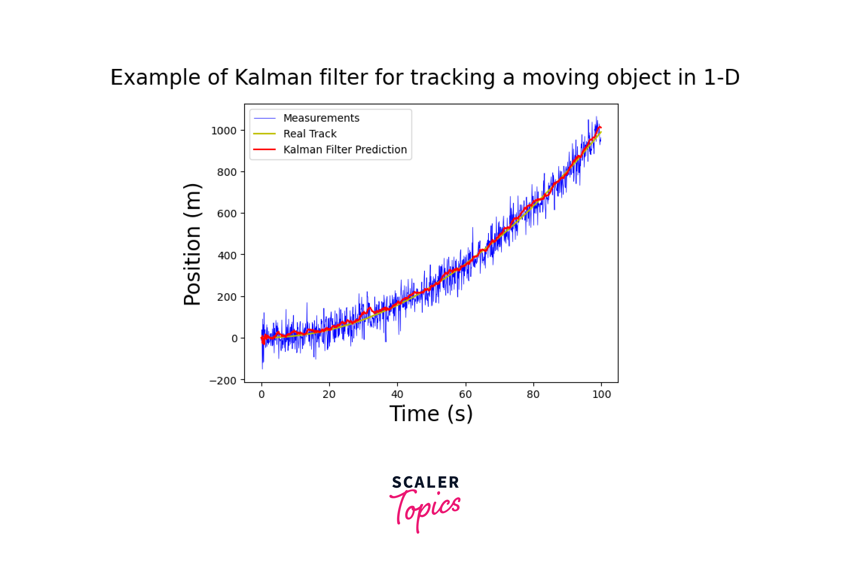
Example of Kalman filter in computer vision for tracking a moving object 1-D
In computer vision, the Kalman Filter can be applied to track a moving object in a 1-dimensional space. The filter combines predicted positions based on a mathematical model with measurements obtained from a sensor, such as a camera. It estimates the object's position and velocity, accounting for noise and uncertainties. By iteratively updating the estimates, the Kalman Filter provides a smooth and accurate tracking of the object's motion in real-time.
Here is the step-by-step implementation of the Kalman filter in computer vision for tracking a moving object 1-D.
Step 1: Importing libraries
The first few lines of the code import the necessary libraries: numpy and matplotlib.pyplot.
Step 2: Defining the KalmanFilter class
The KalmanFilter class is defined with the following methods:
This is the class constructor, which initializes the variables required for the Kalman Filter. The variables initialized include dt which represents the time interval, u which represents the control input, std_acc which represents the standard deviation of acceleration, and std_meas which represents the standard deviation of the measurement.
The function initializes various matrices such as the A, B, H, Q, and R matrices. These matrices represent different properties of the system and are used in the Kalman filter algorithm.
Step 3: Defining the Helper functions
predict(self) and update(self, z) are the helper functions that we will be using here in order to predict the next state and to update the measurement to the Kalman filter.
predict(self) This method predicts the next state of the system using the Kalman filter algorithm. The method takes no arguments and returns the predicted state.
update(self, z) This method updates the Kalman filter based on the measurement received as input. The input parameter z is the measurement received at the current time step. The method updates the state of the system based on the measurement received and returns the updated state.
Step 4: Define the main function The main function is defined which will be used to execute the Kalman filter. The following steps are performed in the main function:
-
Define the time range The time range over which the Kalman filter will be executed is defined using the np.arange function.
-
Define the real track A model track is defined using the equation real_track = 0.1*((t**2) - t). This will be used as the real position of the object being tracked.
-
Initialize the KalmanFilter object An object of the KalmanFilter class is created with the necessary parameters such as time interval, control input, standard deviation of acceleration and measurement.
-
Run the Kalman filter The Kalman filter is run over the time range using a for loop. At each time step, a measurement is received, and the Kalman filter is updated. The predicted state and measurements are stored in lists for plotting.
Output
Applications of Kalman Filter in Computer Vision
Kalman filter is widely used in computer vision applications. Some of the common applications of the Kalman filter in OpenCV are:
Object Tracking
The Kalman filter is extensively used for object tracking in computer vision. In object tracking, the Kalman filter can be used to track the motion of an object over time. The filter predicts the location of the object in the next frame by using the current location and velocity of the object. The predicted location is then compared with the actual location of the object in the next frame. If the actual location is different from the predicted location, the Kalman filter corrects its prediction based on the measurement.
OpenCV provides a variety of functions to perform object tracking using the Kalman filter, such as cv2.KalmanFilter(), cv2.measurementMatrix(), cv2.processNoiseCov(), and cv2.errorCovPost().
![]()
Camera Pose Estimation
The Kalman filter in computer vision can be used to estimate the position and orientation of a camera in computer vision applications. The filter can predict the position and orientation of the camera based on the previous position and orientation and the motion model. The predicted position and orientation can be compared with the actual position and orientation of the camera to correct the filter.
OpenCV provides functions to estimate the camera pose using the Kalman filter, such as cv2.calibrateCamera(), cv2.solvePnP(), and cv2.Rodrigues().
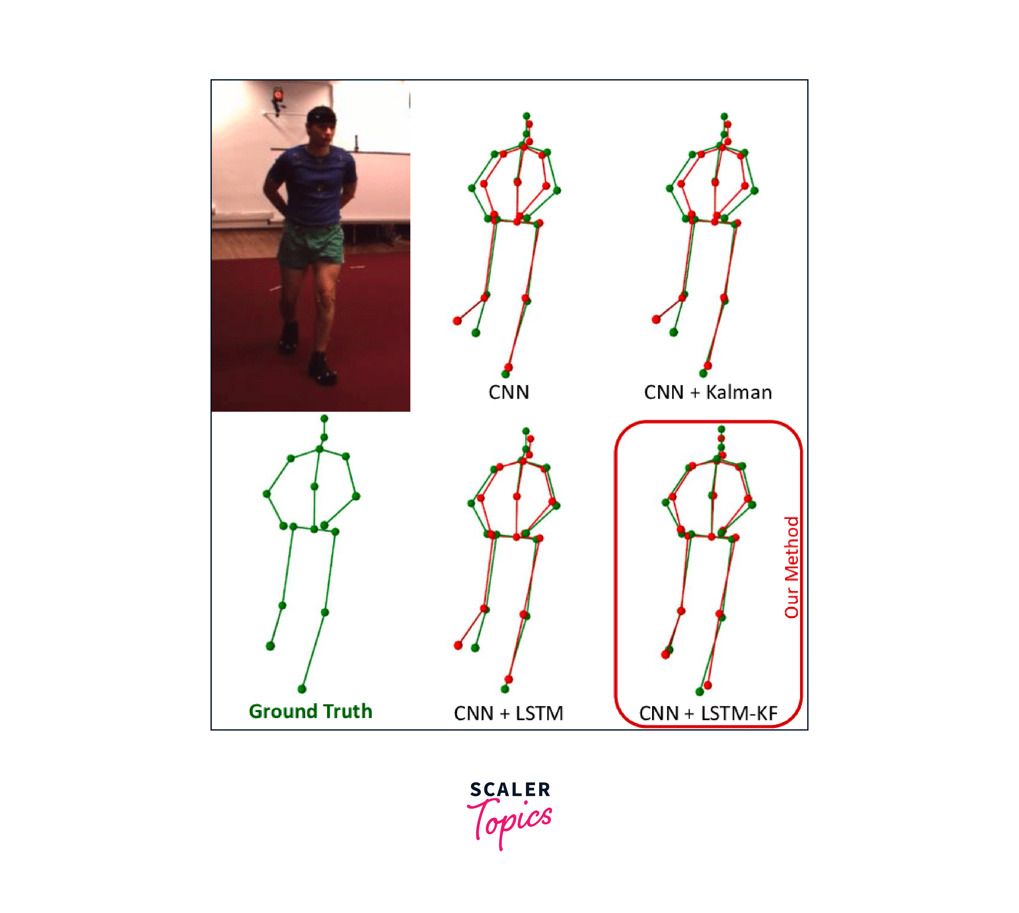
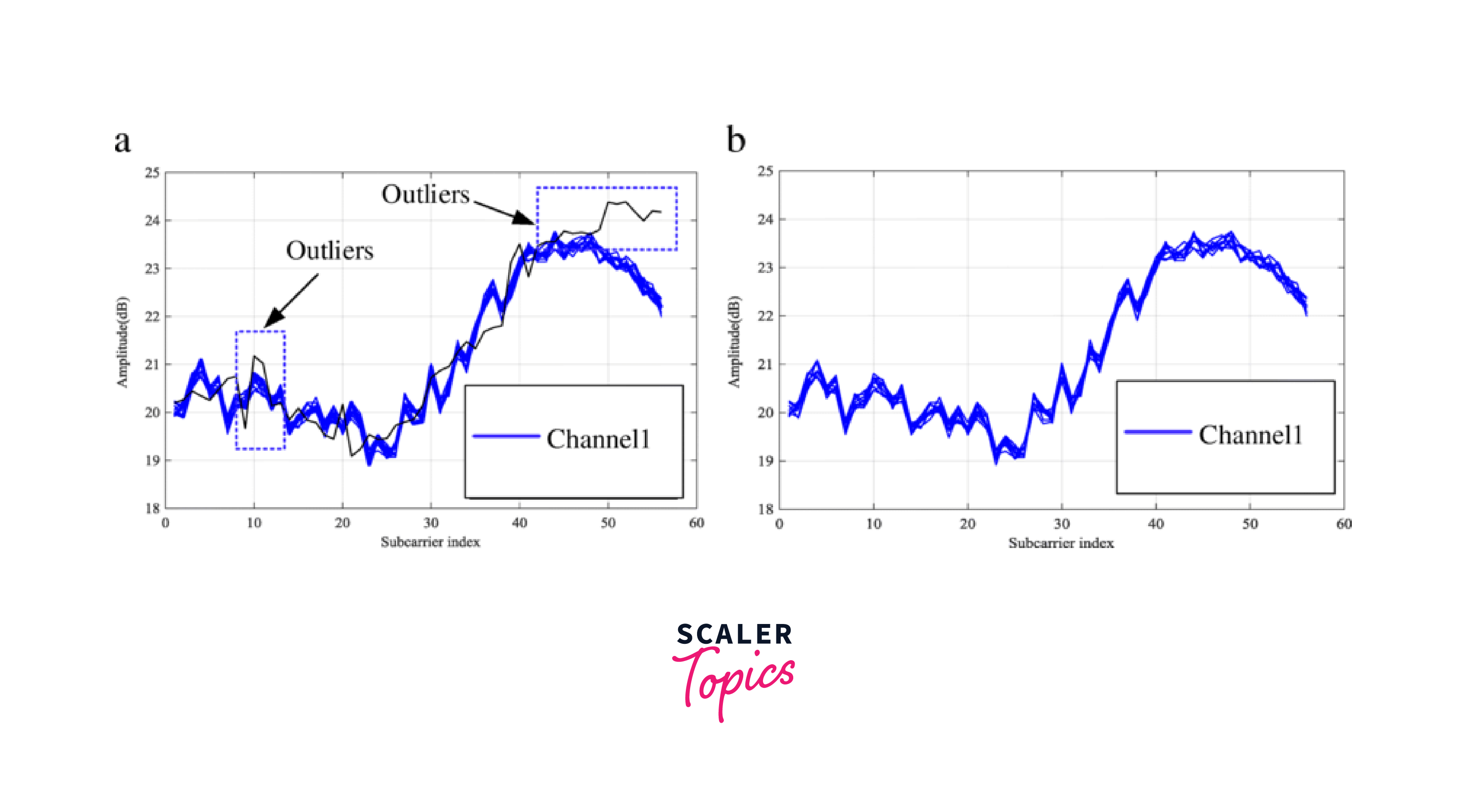
Image Denoising
The Kalman filter can be used to reduce the noise in images. The filter can predict the noise in the image and subtract it from the image to produce a denoised image. The filter can also estimate the noise parameters based on the previous noise levels and the noise model.
OpenCV provides functions to perform image denoising using the Kalman filter, such as cv2.fastNlMeansDenoisingColored(), cv2.fastNlMeansDenoising(), and cv2.fastNlMeansDenoisingMulti().
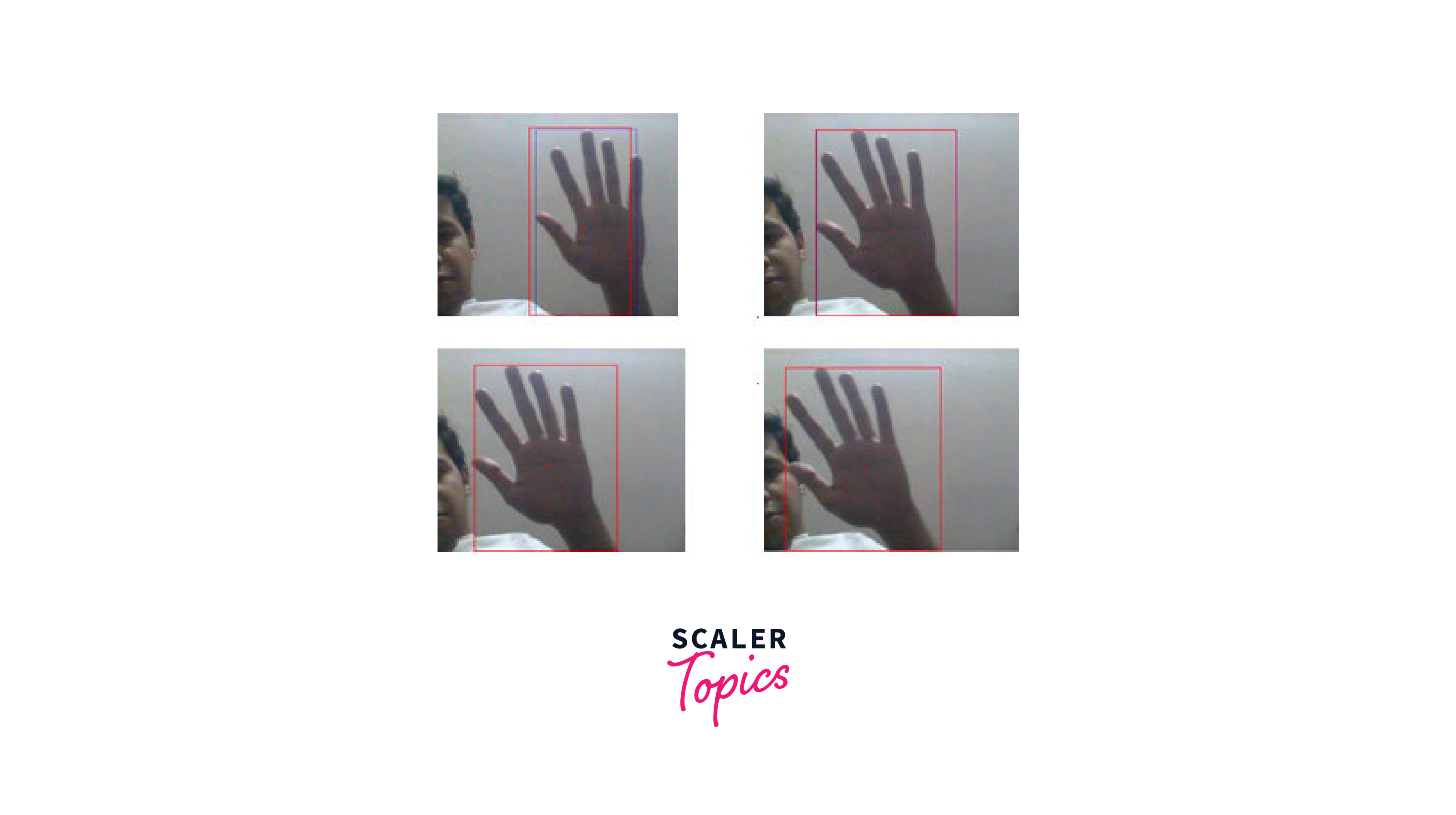
Hand Gesture Recognition
The Kalman filter in computer vision can be used to recognize hand gestures in computer vision applications. The filter can predict the position and velocity of the hand based on the previous position and velocity and the motion model. The predicted position and velocity can be compared with the actual position and velocity of the hand to recognize the gesture.
OpenCV provides functions to recognize hand gestures using the Kalman filter, such as cv2.contourArea(), cv2.convexHull(), cv2.boundingRect(), and cv2.circle().
Comparison of Kalman Filter with other filters in OpenCV
Here's a comparison of the Kalman filter with some other filters commonly used in computer vision applications:
| Filter | Advantages | Disadvantages |
|---|---|---|
| Kalman Filter | Can handle noise, incorporate feedback, fast and efficient | Requires significant computational power, may not perform well with nonlinear or non-Gaussian systems |
| Extended Kalman Filter (EKF) | Can handle non-linear systems, incorporate feedback | Requires significant computational power, may not perform well with highly non-linear systems |
| Unscented Kalman Filter (UKF) | Can handle non-linear systems, more accurate than EKF, requires less computational power | Sensitive to initial conditions, may not perform well with highly non-linear systems |
| Particle Filter | Can handle non-linear systems, can incorporate feedback, requires no assumptions about probability distribution | Requires a large number of particles, computationally intensive, sensitive to initial conditions |
| Moving Average Filter | Simple, easy to implement, can handle noise | May not handle abrupt changes in system, not accurate in non-stationary systems |
| Median Filter | Handles impulse noise, preserves edges | May not handle Gaussian noise well, may not preserve fine details |
| Gaussian Filter | Smoothes image, preserves edges | May blur fine details, may not handle impulse noise well |
Conclusion
- Overall, this article provided an overview of Kalman Filter in computer vision, along with a comparison of Kalman Filter with other filters in OpenCV.
- The information presented here can be useful for those working in the field of computer vision or interested in learning more about data filtering and estimation.
- Kalman Filter is a powerful tool for handling noisy and uncertain data, and incorporating feedback to improve estimates.
- Kalman Filter remains a powerful and widely used tool for data filtering and estimation, but it is important to be aware of its limitations and consider alternative filters when appropriate.
