Training an Audio Classification Model in Keras

What are We Building?

Analyzing and recognizing any Audio, sound, noise, musical note, or another similar type of data to classify them appropriately is known as audio classification. Many different types of audio data are available to us, including acoustic device sound, musical chords from instruments, human voice, and even naturally occurring sounds like birds chirping in the background. In this Project, our goal is to determine whether the sounds coming use a portion of the speech Commands dataset (Warden, 2018), which contains short (one-second or less) audio clips of commands, such as down, go, left, no, right, stop, up and yes implementing Convolutional Neural Network.

Pre-requisites

The pre-requisites for training an Audio Classification Model in Keras include the following:

• Basic knowledge of TensorFlow Data Input Pipeline and its respective functions.
• In-depth knowledge of the Deep Learning framework to create and train the model.

How are We Going to Build This?

Audio classification is one of the greatest fundamental introduction projects for deep audio learning. The goal is to comprehend the waveforms provided in their raw form and transform the current data into a format the developers can use. We may use deep learning models to interpret and evaluate the data by turning an audio file's raw waveform into spectrograms.

Our goal in this Project is to classify the incoming sound created by a Human, i.e., words. We transform the incoming sound signal into a waveform further, it will be converted into the Spectogram.

Convolutional Neural Networks can be used to assess these spectrograms appropriately by building a deep learning model to produce a multi-label classification result because these spectrograms are visual images. The summarized steps of building an Audio Classifier Neural Network in Keras are Data preparation, Model Design, Training, and Evaluation.

Final Output

Here, we will demonstrate the input and output of the trained Audio Classifier Model in this section. Below is a picture of the predicted outcome.

Requirements

• TensorFLow:
  Google's TensorFlow2.x provides basic tools for building and training neural networks. With Keras, you may manipulate different neural network topologies and stack layers of neurons.
• For preprocessing data, we will use TensorFlow I/O, i.e., TensorFlow Input Output Library, which can be installed using the pip install tensorflow-io[tensorflow] command.
• TensorFlow Signal Processing (TF Signal) is a library for signal processing operations in TensorFlow. It provides a collection of tools for building and training machine learning models for Audio and speech processing tasks, such as speech recognition, speech synthesis, and Audio classification.

Training an Audio Classification Model in Keras

In this section, we are going to train the Audio Classifier Model. This is a multi-class classification task where the trained Neural Network will classify the human speech sound. The model will accept the Spectrogram as the input, and based on the features from the Spectrogram, the model will classify the human speech into their respective class. The study of audio signals, sound waves, and other modifications to audio frequencies is known as Audio Signal Processing.

Importing Libraries

We will import all of the necessary libraries in the subsequent step to build the Project. To analyze the generated spectrograms and produce the desired outcome for this Project.

Dataset Preprocessing

You'll be working with a scaled-down version of the Speech Commands dataset to speed up data loading. Over 105,000 Audio files in the WAV (Waveform) audio file format representing humans speaking 35 distinct words make up the original dataset. This information was gathered by Google and made available with a CC BY license.

tf.keras.utils.get_file is a utility function in the TensorFlow library that allows you to download a file from the internet and save it to your local file system. It is commonly used to download datasets or pre-trained models for machine learning projects.

The function takes in several arguments:

• fname: the name of the file to be downloaded.
• origin: the URL from which the file should be downloaded.
• untar: if True, the downloaded file will be automatically extracted (if it's a tar file).
• md5_hash: an optional MD5 hash of the file to check for integrity after downloading.
• file_hash: an optional file hash to check for integrity after downloading.
• cache_subdir: an optional subdirectory to save the file in.
• It returns the local path to the downloaded file.

The file will be downloaded and cached. If the file already exists in the cache, it will use in the cache directory.

We will use tf.keras.utils.get file to download and unzip the mini-speech commands.zip file containing the scaled-down Speech Commands datasets:

Output:

This code uses the tf.keras.utils.get_file function to download a zip file containing a dataset called "mini_speech_commands" from a specified URL. The file is saved to the local file system in a directory called data/mini_speech_commands. The code first checks if the directory data/mini_speech_commands already exists. If not, it proceeds to download the file. The extract argument is set to True, meaning the zip file will be automatically extracted after being downloaded.

The cache_dir argument is set to '.' which means the file will be cached in the current working directory, and cache_subdir is set to data which means that the file will be saved in a subdirectory called data within the cache directory. This way, the next time you run the script if the file already exists in the cache directory, it will use the cached file and not download it again.

Output:

This code snippet uses the TensorFlow (tf) library to access the Google File System (gfile) and list the contents of a directory specified by the variable data_dir. The resulting list of files is stored in the variable commands, which are then filtered to remove the files README.md and .DS_Store using a boolean indexing operation. The final list of commands is then printed to the console.

Eight folders, one for each spoken command in the dataset, are used to hold the audio clips: no, yes, down, go, left, up, right, and stop. The above code snippet uses the TensorFlow (tf) library to create two datasets - train_ds and val_ds, from the Audio files in a directory specified by the variable data_dir. The function audio_dataset_from_directory() is used to create the datasets with the following parameters:

• directory: the path to the directory containing the Audio files
• batch_size: the number of Audio files per batch
• validation_split: the proportion of Audio files to use for validation (the remaining files will be used for training)
• seed: the seed for the random number generator used to split the files between training and validation
• output_sequence_length: the number of Audio samples in each file
• subset: 'both' to return both train and validation datasets.

The resulting dataset will contain the names of the classes and it is stored in the variable label_names, which is then printed to the console as shown below.

Output:

The below code snippet defines a function squeeze that takes two arguments, Audio and labels, and applies the TensorFlow (tf) function tf.squeeze() to Audio to remove size one dimension from the tensor. This function removes the last dimension of the Audio data as it is mono-channel Audio. The axis parameter is set to -1, specifying the tensor's last axis. After the Audio tensor has been modified, the function returns a tuple containing the modified Audio tensor and the original labels tensor.

The squeeze function is then applied to both the train_ds and val_ds datasets using the map() function, which applies a function to each dataset element. The second argument of the map() function is set to tf.data.AUTOTUNE, which tells TensorFlow to use the best performance configuration available on the device. This way, the dataset can be used for training and validation purposes.

The below code snippet uses the shard() function to split the val_ds dataset into two smaller datasets: test_ds and val_ds. The shard() function takes two arguments:

• num_shards: the total number of shards to divide the dataset into
• index: the index of the shard to return.

In this case, the val_ds dataset is being split into two shards for testing and validation by specifying num_shards=2. The index=0 argument is used to select the first shard and assign it to test_ds, and the index=1 argument is used to select the second shard and assign it to val_ds. This way, the dataset is split into two for testing and validation purposes, in the ratio of the shard index.

Converting Waveforms to Spectrograms

In this section, we will have basic knowledge of Spectrogram and how to convert Audio Signal into Spectrograms.

Waveform:

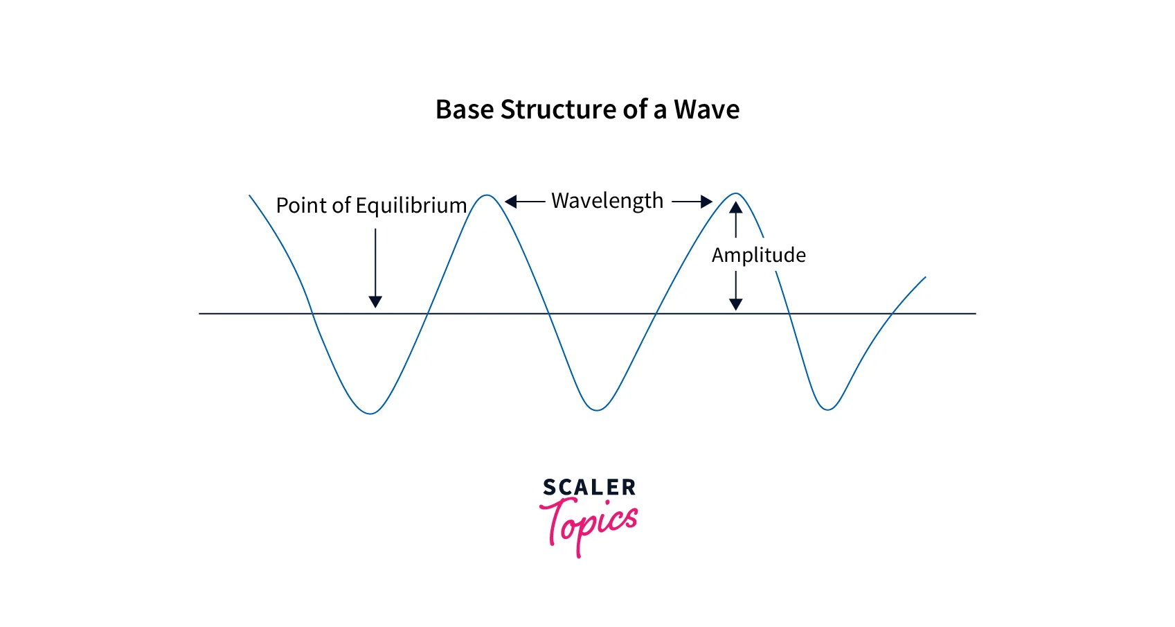
When the air particles around an object vibrate in air pressure, it produces sound waves. Mechanical waves, like sound, carry energy from one source to another. A waveform is a schematic illustration that facilitates the analysis of the displacement of sound waves over time and certain other crucial variables needed for a particular activity.

Spectograms:

The visual representation of the Audio signal's frequency spectrum is called a spectrogram. Sonograph, voiceprints, and voicegrams are other technical names for spectrograms. These spectrograms are widely employed in various fields, including speech recognition, audio classification, linguistic analysis, music creation, and signal processing. In this post, we'll also employ spectrograms for categorizing Audio.

The dataset's waveforms are displayed in the time domain. Next, we will compute the short-time Fourier transform (STFT) to turn the waveforms into spectrograms, which may be seen as 2D images and show frequency changes over time. These spectrograms will display frequency changes over time. We will feed the spectrogram images into your neural network to train the model.

A signal is broken down into component frequencies using the Fourier transform (tf.signal.fft), but all temporal information is lost. In contrast, STFT (tf.signal.stft) divides the signal into time windows, performs a Fourier transform on each window, and returns a 2D tensor that can be used with normal convolutions.

Make a useful function that transforms waveforms into spectrograms:

1. The waveforms must be the same length for the resulting spectrograms to have equal dimensions. Simply zero-padding the Audio segments under one second will accomplish this (using tf.zeros).
2. Choose the frame length and frame step arguments when calling tf.signal.stft so that the resulting spectrogram "image" is nearly square. Refer to this Coursera video on audio signal processing and STFT for more details on selecting STFT parameters.
3. The STFT generates an array of complex integers that represent magnitude and phase. You can calculate the magnitude by applying tf.abs to the tf.signal.stft output will only be used in this lesson.

The above code snippet defines a function get_spectrogram that takes a 1-D tensor waveform as input and converts it to a spectrogram. The function performs the following steps:

It uses the TensorFlow (tf) function tf.signal.stft() to perform a short-time Fourier transform (STFT) on the input waveform. The frame_length and frame_step arguments are set to 255 and 128, respectively, the window size and the step size used for the STFT.

It obtains the magnitude of the STFT by taking the absolute value of the complex-valued STFT using tf.abs(). Then, it adds a new dimension to the Spectrogram with tf.newaxis so that the Spectrogram can be used as image-like input data with convolution layers. It returns the Spectrogram. The output of this function is a complex-valued tensor of shape (batch_size, time, frequency, 1), which can be used as input for convolution layers.

Plotting Spectrograms with Waveforms

The above code snippet defines a function plot_spectrogram that takes a 2D tensor spectrogram and an axis ax as input and plots the Spectrogram using the pcolormesh() function from the matplotlib library.

The function performs the following steps:

1. It checks if the Spectrogram has more than two dimensions, and if so, it uses the numpy function np.squeeze() to remove the last dimension if its size is 1.
2. It converts the frequency axis of the Spectrogram to log scale, as a logarithmically spaced frequency axis gives a better perception of the amplitude.
3. It transposes the Spectrogram so that the time is represented on the x-axis (columns)
4. It adds a small positive number to the Spectrogram to avoid taking a log of zero.
5. It creates a mesh grid of X and Y to plot the Spectrogram.
6. It plots the Spectrogram using the pcolormesh() function.

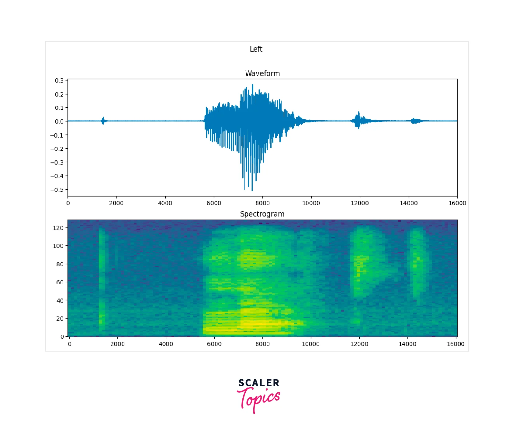
The resulting plot is a 2D representation of the input audio, where the x-axis is time, and the y-axis is frequency, with the amplitude represented by color. After executing the above code, the following output can be seen as a graph below.

The below code snippet defines a function make_spec_ds that takes a dataset ds as input and applies the get_spectrogram() function to the Audio in the dataset, returning a new dataset containing the spectrograms.

The function uses the word map() function on the input dataset ds and applies the lambda function to each element. For example, the lambda function inputs an audio and label and returns a tuple of the Spectrogram of the Audio and the label. The number of parallel calls is set to tf.data.AUTOTUNE, which tells TensorFlow to use the best performance configuration available on the device.

This way, the dataset is transformed into spectrogram data that can be used for training or validation purposes.

This code uses the TensorFlow (tf) data module to preprocess a dataset called train_spectrogram_ds. It first caches the dataset in memory, then shuffles it using a buffer size of 10000, and finally prefetches the next batch using the AUTOTUNE option. This can improve the performance of the training process by reducing the time spent loading data and allowing the model to start training on the next batch while the current one is being processed. Same process is implemented for test_spectrogram_ds and val_spectrogram_ds

Model Creation and Training

In this section, we will create and train the Audio Classification Model. The below code defines a neural network model using the Sequential class from the Keras library. The model comprises a stack of layers, each representing a transformation of the input data.

First, a 2D convolutional layer (Conv2D) is added to the model with 16 filters of size $3x3$, using the ReLU activation function, with input_shape of (124, 129, 1). This layer is used for feature extraction from the input image.

Then, another 2D convolutional layer is added with the same filters and activation function size. This layer is also used for feature extraction. Next, a Flatten layer is added, reshaping the previous layer's output into a 1D array. Then, a Dense (fully connected) layer is added with 128 neurons and a ReLU activation function. This layer is used for the classification of the extracted features. Finally, a Dense layer is added with eight neurons and a softmax activation function. This layer will output the probability of each class.

The model.summary() function call at the end of the code will print a summary of the model architecture, including the number of parameters in each layer.

Once the model architecture has been built, we may compile and train the model appropriately. The Adam optimizer, the binary cross-entropy loss function, and additional recall and accuracy metrics can all be defined for the model analysis and construction. Finally, we can fit the model for a few epochs by training the previously constructed data using the validation test data. Below is a code snippet that demonstrates the outcome of this step.

Output:

Making Prediction on a Single Sample

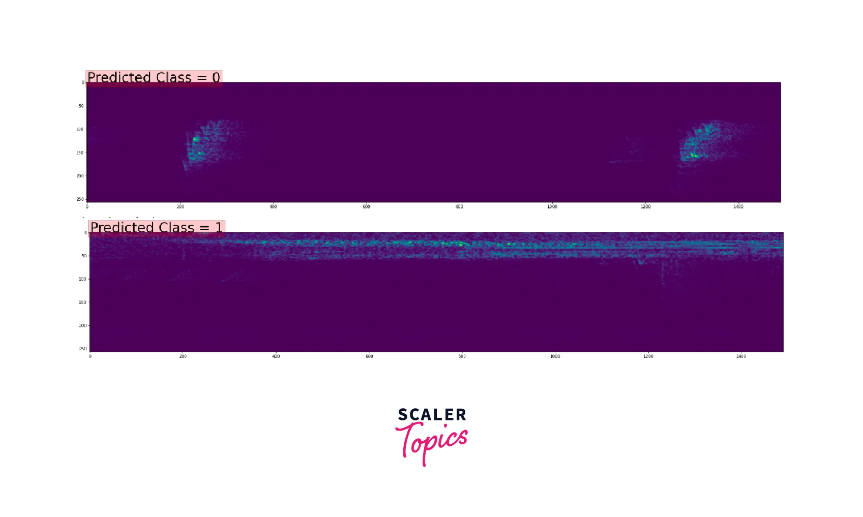
After successfully building and training the model, we may examine and validate the outcomes. The measures found in the results demonstrate good development. The model we've created is appropriate for producing reasonably accurate predictions on the samples of mini_speech_commands. The code snippets are shown below.

In the code snippets below, we plot the input images with the output label. So you have a clear idea of how to plat the input images with the predicted label as well as the whole process of Prediction. We are showing a few plotted images, but if you run the code snippets, it will plot the whole test set with the predicted labels.

What's Next?

In this article, we have developed and trained an Audio Classifier Model using Spectrograms. It is like an Image Classification model where we can classify the Spectrograms. Raw Audio Signals can be fed directly into the 1D-Convolutional Neural Networks for classification. Also, we can use Attention Networks with Convolutional Neural Networks to classify the Audio Signals.