Distributed Training for Customized Training Loops in Keras

Introduction

Deep Learning (DL) models are data-hungry, meaning they need large data for training and weight optimization. Nowadays, we see models with billions of parameters, such as GPT-2, ChatGPT, and various other models. The larger the Model, the larger the computational time while training the Model. So we need to use GPUs while training the Model, which can decrease the computational time. In this article, we will study how to train the Model by utilizing all the GPUs available on the system. By default, TensorFlow utilizes only 1 GPU if it is available.

Training a Classification Model on GPU with Custom Loop

Training your models on a single CPU and GPU unit may become impossible as they become more complicated. As a result, you might need to devise a strategy for dividing training across several instances or GPUs. Tensorflow has devised several approaches to accomplish this.

• First, we can divide our data among multiple computers or instances. Each cluster may have one or more machines that may train your models extensively as necessary. One may refer to this as a distribution strategy. In Keras, a custom training loop can be implemented by creating a subclass of the tf.keras.Model class and override the train_step() method. This method is responsible for performing the forward and backward pass of the Model for a single training step, and it can be customized to include any additional operations that are required.
• The second approach is dividing the model structure into the available GPUs and training the full neural network by splitting the layers over the different resources or GPUs.

This article will show you how to train a Classification Model with a Custom Training Loop on the available GPU.

Step 1: Importing the required libraries

The required libraries must first be imported. To enable the implementation of the classes and functions in our code, shown below.

Step 2: Data Loading and Data Preprocessing

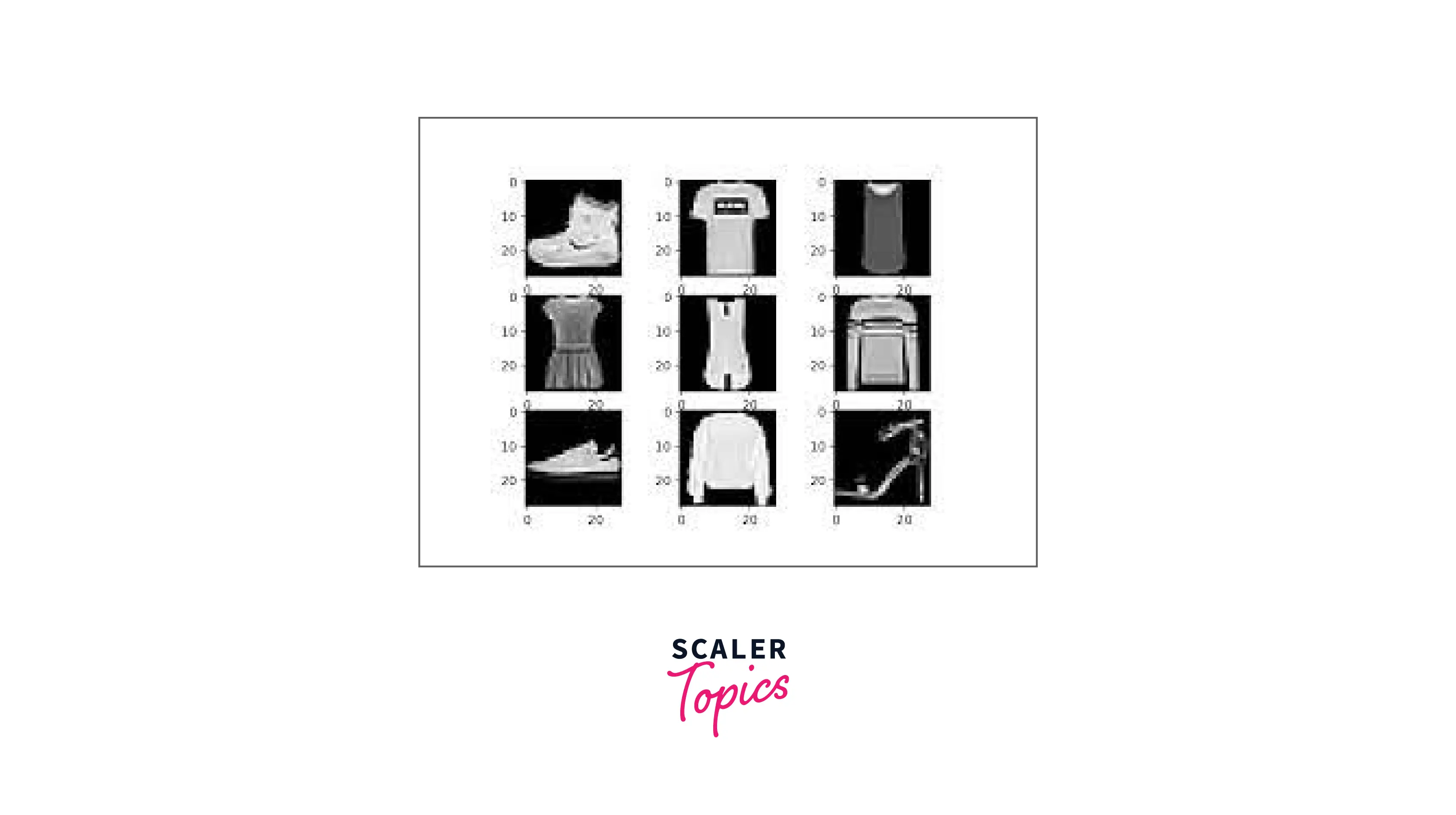
To explain this article, we have utilized the Fashion-MNIST dataset, which comprises 70,000 images of 10 output classes like T-shirts/tops, Trousers, Pullovers, Dress, Coat, Sandal, Shirt, Sneaker, Bag, and Ankle boots. These data points have values in greyscale for each image and comprise only one channel. The dataset is already split into train and Test splits, so we don't have to do any train_test split explicitly. The train set consists of 60,000 images and the test set consists of 10,000 images.

• The dataset is scaled by dividing each pixel by 255, resulting in a range of values for each pixel between 0 and 1.

• We will be using the Convolution Neural Network 2D model, so the dataset will be preprocessed via normalization, transforming the labels into categorical values and reshaping the dataset into a 28,28,1 shape.

The preprocessing step of the MNIST Fashion dataset is shown in the code snippets below.

Dataset Shape and Samples are shown below:

Output:

Step 3: Distribution Strategy

There are various Distribution Strategies available in Keras and TensorFlow:

• tf.distribute.experimental.MultiDeviceStrategy: It is a TensorFlow API for distributing training across multiple devices and machines. It allows you to run your training on multiple GPUs, either on one machine or multiple machines in a network. With this strategy, you can scale up your training to handle larger models or batch sizes, thus speeding up the training process.
• tf.distribute.experimental.ParameterServerStrategy: A TensorFlow distribution strategy allows multiple replicas to run on the different physically separated systems while sharing a set of parameters stored on one or a small number of parameter servers.
• tf.distribute.MultiWorkerMirroredStrategy: It s a TensorFlow API for distributing training across multiple workers, each with multiple GPUs. It uses collective communication to synchronize gradients and maintain consistency of variables across all replicas. This strategy enables training on large-scale, multi-node clusters and can significantly speed up the training process by leveraging the power of many GPUs.
• tf.distribute.MirroredStrategy: It is a TensorFlow distribution strategy that supports synchronous training on multiple GPUs on one machine. With this strategy, each available GPU in a single system has a copy of the Model, and gradients are aggregated across the replicas before being applied to the parameters. This increases training speed and improved model accuracy as the data is split across multiple GPUs. The MirroredStrategy supports multiple synchronization methods to handle the aggregation of gradients, including "synchronous" and "asynchronous" methods, and can be used for single-worker and multi-worker training. For this exercise, we will be using tf.distribute.MirrorStatergy().

tf.distribute.MirrorStatergy will perform Data parallelism, allowing us to train our Model on different batch samples on multiple GPUs. These GPUs instances will have copies of the model parameters that are used for training and are referred to as replicas. The below steps explain the tf.distribute.MirrorredStratergy :

1. A model is created and replicated across all available GPUs.
2. The data is split into smaller batches, each assigned to a replica for processing.
3. Each replica processes its assigned batch and computes the gradients concerning the Model's variables.
4. Depending on the user's configuration, the gradients are aggregated across all replicas, either by summing or averaging.
5. The aggregated gradients update the Model's variables in sync across all replicas.
6. The updated Model is then ready for the next batch of data.

This process repeats until the end of the training process, providing faster training time than single-GPU training, as multiple GPUs can process different batches simultaneously.

Below, I have mentioned the summarized steps on how to use Distributive Training Strategy using Custom Loop:

1. Initialize tf.distribute.MirroredStrategy
2. Distribute tf.data.Dataset
3. Perform Loss Calculation and aggregation per replica.
4. Initialize models, optimizers, and checkpoints with tf.distribute.MirroredStrategy
5. Distribute computation to each replica
6. Aggregate returned values and metrics

Output

As we can see, I have 2 GPUs in my system. Similarly, in your system, if you have one or more than one GPU, the Distribute Strategy will take it on its own; we do not need to specify the GPU number explicitly.

We have 2 GPUs available, so we will feed an equal number of samples to each of the GPUs so that the Model can perform Forward and Backward Propagation, which will optimize the model weights. Therefore, I have initialized the batch size of 64 under the variable name BATCH_SIZE_REPLICA this will be the batch size of one GPU instance.

We multiply the GPU instances with the BATCH_SIZE_REPLICA variable known as GLOBAL_BATCH_SIZE. The Model will receive the GLOBAL_BATCH_SIZE as input, but it will divide the GLOBAL_BATCH_SIZE by the number of GPUs instances available, and it will feed the resultant batch size to all the replicated model instances for training.

Step 4: Creating the Data Pipeline

The Keras API has built-in functionality known as Data Input Pipeline. It is the most efficient way to train models on multiple devices/systems. Data Input Pipeline also helps us to deploy the trained models easily.

In this section, we'll build a data pipeline that will perform the following task:

batch(): The number of training samples used in a single iteration is the batch size in machine learning.

The batches of data samples supplied to the fit function during model training are created using the batch function.

shuffle(): The dataset is shuffled using the shuffle function.

map(): The dataset's samples are preprocessed using the map function. Then, the lambda function or a custom/TensorFlow function can be called from within the map function. The function will process all of the samples in the dataset, and each sample will be processed individually.

Prefetch(): It keeps the next batch or batches ready to be immediately available once the GPU completes its iterations of the current batch while working on forward and backward propagation. We can apply this idea in cases where the GPU consumes, and the CPU produces cached datasets. All that is necessary is to ensure that at least one batch is always available so that GPU could be better.

Here, I have created two input data pipelines using tf.data: one for training data and the other one for test data.

After creating the Data Input Pipeline, we must distribute the testing and training dataset. The below code displays how we can distribute the Test and Train Dataset on the number of GPUs available on the system.

Step 5: Visualization of the Dataset

In this section, we will visualize the train and test dataset.

Output:

Step 6: Creating the Model Architecture

I have created a basic 2D-Convolutional Neural Network (CNN) model to make things easier (CNN).

The neural network expects the above dataset to be in a specific shape. Therefore, when training models with Keras, we pass the shape as image_width, image_height, and number_of_channels. Failure to do this will result in an error such as ValueError: Exception Input 0 of layer "conv2d" is incompatible with the Layer: expected min_ndim=4, found ndim=3.

Input Layer: The first Layer of the Model is the input layer, which provides the dataset's input shape as Nonex28x28x1 which includes the total number of samples in the batch, the image's height and breadth, and the number of image channels.

Convolutional Layer: The model architecture also constitutes two Convolutional Neural Network Layers (CNN) with feature maps of 64 and 128 with a kernel size of $3*3$, respectively.

Max Pooling Layers: The maximum pooling layer with a pooling size of $2*2$ has been added after each convolutional neural network layer. The feature maps obtained from the Convolutional Neural Network will be down-sampled since the Max Pooling layer will extract the most value from the feature map patches.

Dropout Layers: A dropout layer with a probability of 0.5 means that to prevent overfitting, 50% of the Layer's neurons will be randomly deactivated during training.

Classification Layer: The Classification Layer is the last layer of the Model. This Layer has ten neurons since we need to categorize ten different objects. It comprises the activation function known as Softmax, which outputs the probability of the classes linked with the datapoint and has a range between 0-1.

After creating the Model architecture, we have just wrapped it under the function named created Model.

The code snippets for the Model are shown below:

Here, a Model summary can be printed using the .summary() method, which shows total, trainable, and non-trainable parameters, the name of the layers, and each layer output shape.

Output:

Step 7: Custom Training Loop

Customized training loops offer more coding freedom, the ability to incorporate new logic, and complete control over the entire training process. For more detail, please refer to the article on Custom Training Loop Using Keras Dear SEO Team, Please add the link to the Customized Training Loop in Keras.

Loss Function

In this section, we will define the loss function. We will use CategoricalCrossentropy because the labels are one hot encoded. If labels are not one-hot encoded, SparseCategoricalCrossentropy is used instead. The goal is to reduce the errors between the true and predicted values. The CategoricalCrossentropy function takes probability predictions and returns the average Loss. We have used from_logits to False because we have created a model so the classification layer has a Softmax activation function.

Let's assume that each replica of a batch of input distributed across two GPUs has a size 64 input. When each Model calculates the forward propagation loss, it is split by GLOBAL_BATCH_SIZE, rather than 64. Because each Model calculates gradients, this method must sync the gradients across all models by adding them together.

When implementing a custom training loop, keeping track of the per-example loss values and properly scaling them to obtain the final loss value for the entire batch is important.

One way to do this is to add up all the per-example loss values using the tf.reduce_sum() function and then divide the total by the global batch size, the total number of examples in the batch. This can be done using the following line of code:

Alternatively, you can use the tf.nn.compute_average_loss() function, which automatically computes the average Loss for a batch of inputs and weights. This function takes the per-example loss values and the number of elements in the batch as arguments.

Both of the above methods are equivalent and return the average Loss for the batch. It's up to you which one to use, depending on your specific use case and implementation.

When creating a custom training loop for a model with additional losses, such as regularization losses for weights, it's important to consider these losses when computing the final loss value for the batch. This can be done by adding up all of the losses, including the per-example and regularization losses, and then dividing the total by the number of replicas.

To achieve this, you can use the tf.nn.scale_regularization_loss() function. This function takes the regularization losses as an argument and returns the scaled regularization loss. This can then be added to the per-example Loss to obtain the final loss value for the batch. Here's an example of how this can be done:

It's important to note that the tf.nn.scale_regularization_loss() function will divide the regularization loss by the number of replicas. It will also multiply the Loss by the weight decay, in case you are using a weight decay optimizer. This is a more advanced feature, and it's recommended to have a good understanding of the underlying concepts of training neural networks and regularization techniques.

When training a model using a custom training loop, it's important to be mindful of the batch size and how it may affect the final loss value.

If the training data permits it, it is possible to have batches that are smaller than the global batch size—in this case, using the tf.reduce_mean() function to compute the average Loss over the actual batch size can lead to instances of small batches being overweighted. Instead, it's a best practice to divide the prediction loss by the global batch size to ensure that instances from small batches are not overweighted. This can be done by multiplying the per-example Loss by (1. / GLOBAL_BATCH_SIZE).

It's important to keep in mind that this could lead to larger losses for small batches, which can affect the Model's performance. Therefore, make sure the data is properly shuffled, and the batch size is chosen appropriately. It's also important to note that this is a more advanced feature, and it's recommended to have a good understanding of the underlying concepts of training neural networks and batching strategies.

The below code displays the process of creating the Loss function, which will aggregate the Loss from all the GPU instances and apply it to all the replica of the Model in the GPU.

Creating Matrices

These measures monitor test accuracy, test loss, and training accuracy.

Training Loop

Here, we define the Model and optimizer under the scope of the distribution strategy. An optimizer function uses the computed gradients to adjust the model weights and biases to minimize the Loss. This iterative process aims to find the model parameters that result in the least error. We apply the Adam optimizer function. Adam was selected as an optimizer to propagate the error backward. Adam is a combination of the Root Mean Square Propagation (RMSProp), Adaptive Gradient Algorithm(AdaGrad), and Stochastic Gradient Descent.

The code is shown below:

The training loop feeds the training images to the network while computing the metrics. We have used the Categorical_Accuracy to compute the accuracy because the labels are one hot encoded. The breakdown of the Training steps is shown below:

• Pass the training data to the network for one epoch.

• Obtain the training images and labels for each batch.

• Activate the Gradient.tape()

• Predict the Model by passing the dataset into the Model

• Calculate the Loss by computing Categorical_Crossentropy from prediction and labels

• Deactivate the Gradient.tape()

• Calculate the gradient

• Update model parameters using the Adam optimizer.

• Calculate the metric value and update the respective metric for visualizations.

• Repeat the process for the specified number of epochs.

After the end of the epoch, we are also evaluating the Model so that we have an idea about the model performance after every epoch. That is why I am Validating the Model after every epoch. The process of the model validation on the Test dataset is shown below:

• Pass the testing data to the network
• Predict the Model by passing the dataset into the Model
• Calculate the Loss by computing Categorical_Crossentropy from prediction and labels
• Calculate the metric value and update the respective metric for visualizations.
• Repeat the process for the specified number of samples in the dataset.

The custom training loop snippets are designed to create a tensorflow graph by implementing @tf.function, shown below in the code snippets, @tf.function decorator on computationally intensive tasks. This will compile decorated functions into a callable TensorFlow graph which will be executed faster compared to eager execution.

The functions named distributed_train_step and distributed_test_step will train and test the Model with the Distribution Strategy discussed above and apply the gradients to the Model's replicas in the available GPUs.

The code uses the tf.function decorator to create a distributed_train_step function that runs the training step across multiple devices using the specified distribution strategy. The strategy.run() method is used to run the training step on each device. The Strategy.reduce() method reduces the per-replica losses and computes the final loss value.

The distributed_test_step function is also decorated with tf.function, running the test step across multiple devices. The strategy.run() method runs the test step on each device.

The training loop then iterates through the distributed training dataset, calling the distributed_train_step function to perform the training step and accumulate the total Loss. Finally, the test loop iterates through the distributed test dataset, calling the distributed_test_step function to perform the test step.

After each epoch, the code prints out the current Loss, accuracy, test loss, and test accuracy. The train_accuracy, test_loss, and test_accuracy are the metrics used to track the model's performance during the training and test step.

It's important to note that this is a more advanced feature, and it's recommended to have a good understanding of the underlying concepts of distributed training and TensorFlow's tf.distribute API.

After training the Model, we can see in the output section that the batches of the data are fitted into the Model, and the Model's Loss decreases after each epoch.

Output

For saving the Model, we can create Model Checkpoints and save it after the specified interval. For loading the model checkpoint, we do not require a distribution strategy. The model checkpoint can be loaded with or without the Distribution strategy and can be used to predict the new data points.