Introduction to Transfer Learning in Keras
Overview
In this article, we will study Transfer Learning in Keras. Transfer Learning was a breakthrough in the field of Artificial Intelligence. It solved the problem related to Data Shortage while training any Deep Learning (DL) model. This article focuses on implementing the Transfer Learning Models in Keras on the CIFAR-10 Dataset.
Pre-requisites
To excel in this article, the end user should have intuition about the Keras Model API and the Sequential Model API.
What is Transfer Learning?
Transfer Learning is the process by which we transfer the knowledge of one model to another to solve a particular problem. For example, researchers and Scientists have trained state-of-the-art models such as VGG and its version, Densenet and its version, Inception and its and many other models, which can be found here. We can leverage these trained and optimized models to solve our problem using their weights or architectures. Furthermore, since these models are already trained and optimized, we will have lower training time and can also be trained on small datasets.
It was one of the breakthroughs that enabled many researchers to transfer the features learned by the trained model into their model and fine-tune the new model concerning their small datasets. Scientists/Researchers have found a way by which we can use the per-trained models to train the new neural network architecture.
Transfer learning for machine learning is when existing model components, such as weights or architecture, are reused to solve a new problem statement. Transfer learning is not a machine learning algorithm but a process to train the model using another baseline model. The knowledge developed from previous training is reused to solve new problem statements. Still, the new task will be related in some way or another to the previously trained task, which could be to categorize objects in a specific file type. Transfer Learning can be used with the following section of Machine Learning, which is mentioned below:
- Transfer Learning in Natural Language Processing.
- Transfer Learning in Computer Vision.
- Transfer Learning in Neural Networks.
- Transfer Learning in Explainable Artificial Intelligence.
- Transfer Learning in evaluating the performance of a Generative Adversarial Network.
Why Transfer Learning?
Transfer Learning was a significant breakthrough because it enabled us to train the model using the weights of pre-trained/optimized models. Below is the reason why we should use Transfer Learning:
-
Model can Be trained on small training samples: Deep Learning (DL) is data hungry, i.e., they need vast amounts of data to optimize the model weights. However, in a practical scenario, there are other options than collecting huge amounts of data. But with Deep Learning, we can also train our Deep Learning (DL) model with small training.
-
Less Training Time: Since the weight of the Transfer Learning Model is already optimized, the training time for models with pre-trained weights will be less when compared to training the model with the random weight value.
-
Less Hardware Resources: The weight of the Transfer Learning Model is already optimized so that we can train only the fully connected layer, and the output of the model will be up to the mark if the Dataset is somewhat similar to the Dataset on which the pre-trained model was trained. However, if the Dataset differs, we can train a selective layer of the Network or whole to achieve the required result.
-
Generalised Approach: Transfer Learning is a more generalized approach to machine problem solving, leveraging different algorithms to solve new challenges.
Why does Transfer Learning Work So Well?
As I have discussed above, Transfer Learning is transferring knowledge from one model to another. The reason why Transfer Learning works so well is discussed below:
-
By using pre-trained weights: The weights of the pre-trained model are already optimized in the Imagenet Dataset or on some other dataset. We can directly use that weight for prediction if our Dataset is similar to the Dataset on which the pre-trained model was trained.
-
By using weights as initializer: The weights of the pre-trained model are already optimized in the Imagenet Dataset or on some other dataset. We can directly use the pre-trained weight as a weight initializer in our model, and we can optimize the pre-trained weight by our Dataset while training all the layers present in the model.
-
Using pre-trained model architecture: The scientist and Researcher have designed the pre-trained Neural Network Architecture after analyzing all the parameters. So if our Dataset is different from the Dataset on which the pre-trained model has been trained in that case, we can use the model architecture and train with our Dataset.
-
Using Transfer Learning Model as a feature extractor: Convolutional Neural Network extracts the feature from the images and then tries to associate the respective class by passing it through a Fully Connected Dense Layer. We can use a Pre-Trained neural network to extract the feature from the object and train Machine Learning (ML) models or Deep Learning (DL) models based on these features.
As I have discussed, every aspect of the pre-trained model is useful in one way or another, which is why transfer learning works well in almost every scenario.
Types of Pre-trained Models Used for Transfer Learning
Researchers have trained many Transfer Learning Models which have their specialties. In this section, I will be discussing some of the pre-trained neural networks which have major impacted the Deep Learning Model architecture below:
| Model Name | Size | Top-1 Accuracy | Top-5 Accuracy | Depth | Parameter | Speciality | Link |
|---|---|---|---|---|---|---|---|
| Xception | 88 MB | 79.0 % | 94.5% | 81 | 22.9 M | Depth-wise Separable Convolution Neural Network (CNN) | Paper Link |
| VGG -16/19 | 528/549 | 71.3%/71.3% | 90.1%/90.1% | 16/19 | 16/19 M | Pioneer in Creating very Deep Neural Network Model (DNN) | Paper Link |
| Mobilenet V2 | 14 MB | 71.3% | 93.6% | 105 | 3.5 M | Pointwise and Depth Wise separable Convolution Neural Network | Paper Link |
| Resnet50 | 98 MB | 74.5% | 92.1% | 25.6 M | 107 | Problem of Vanishing Gradient | Paper Link |
| Densenet-121 | 33 MB | 75.0% | 92.3% | 242 | 8.1 M | Strong Gradient Flow and More Diverse Features maps | Paper Link |
All these pre-trained models were trained on were released from the competition known as ImageNet Large Scale Visual Recognition Challenge (ILSVRC). ILSVRC is an annual Computer Vision (CV) competition on a publicly available dataset called ImageNet. In this section, I have covered a very small subset of the pre-trained model and its specialty. For more detail, please refer here
When to Apply Transfer Learning?
Transfer Learning can be applied in many scenarios. The most widely used case is mentioned below:
- When training data are scarce.
- When Resources are scarce.
- When we have time restrictions for developing models from scratch.
- When we have a huge Dataset.
- Improved baseline performance of the model
Transfer Learning Workflow
Transfer Learning is a mechanism just like a spanner designed to open bolts, but by slight modification, i.e., replacing its head, we can also use it as a hammer. Similarly, we can use the per-trained model to build a new model in the following ways:
- Freezing all layer weights of pre-trained weight and using a fully collected layer of our own.
- By using the architecture of state-of-the-art models without weights with or without default Fully Connected Layers.
- Set some weights of the pre-trained model to trainable with a custom Fully Connected Layer.
- Using the weight of the per-trained modes as an initializer in our custom model.
Freezing Layers: Understanding the Trainable Attribute
When we say Transfer Learning, our minds spark with the intuition of transferring knowledge from one model to another. In Transfer Learning, we can set the parameter to train the specific layer weight or use it as it is. Freezing layers refers to the trained model we will use as our base model will not be trained, i.e., its weights will not be updated. The backward propagation of the error will take place for the layers we have defined in the model architecture, not for the base/pre-trained model or layer. In short Freezing, layer means that the layer weights of the trained model do not change when reused on a subsequent downstream mission. They remain frozen. When backpropagation is performed during training, these layer weights aren't compromised.
The Recursive Setting of the Trainable Attribute
In Transfer Learning, we set the weight of the pre-trained model layers, i.e., the layer has already been trained on some dataset to solve similar problem statements. We have the option which is based on the model performance, resources we have, i.e., computing power, number of training samples, as well as time to set the layer trainable parameter to True, which will indicate that the weight so the layer/ layers will be updated while training the model it will signify that the weight of the pre-trained model is just used as the weight initializer for the model layer or we can set to False which will specify that the weight of the layer/ layers will not be updated at any cost the model will be utilizing the original value if the weight for predicting on the samples.
Fine-Tuning in Transfer Learning
The process of fine-tuning a network entails altering the parameters of a previously trained network to adapt to the upcoming task. The first layers of the Network learn very broad features, and as we move up the Network, the layers tend to learn patterns that are more specific to the task they are being trained. As a result, when it comes to fine-tuning, we want to freeze or preserve the initial layers while retraining the subsequent layers to perform our task. There are two reasons why training only requires a small amount of data. First and foremost, we are only instructing some of the Network. Second, the part being trained needs to be taught from the ground up. The time required will also decrease due to the fewer parameters that need to be updated.
All the Transfer Learning Models are trained on the Imagenet Data, which consists of 1000 objects and 14,197,122 annotated images. These pre-trained model weights are optimized for this Dataset only. Therefore, if we want to use the weights of these pre-trained models or the architecture, we must change the model per our requirements.
Model Architecture:
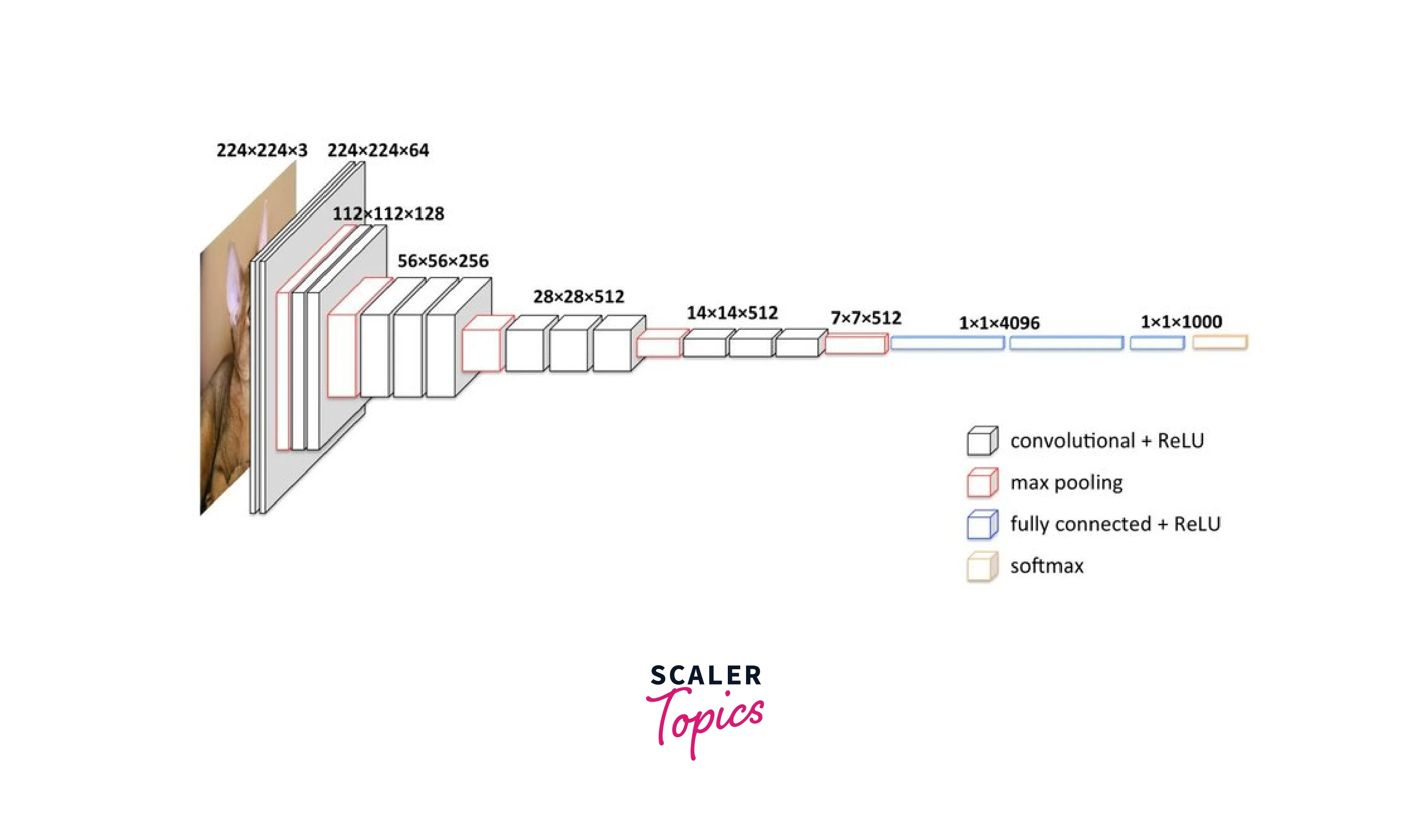
As we already know, the number of neurons in the classification layer depends on the number of objects we want to classify. The pre-trained neural Network is trained on the Imagenet Dataset, which consists of 1000 objects. Suppose the number of objects we want to class equals the number in the Imagenet Dataset. In that case, we can proceed as it is, but if the number of objects varies, we must implement our Dense Layer by the Dataset and optimes the weights of the Fully connected Layer only. The below image describes the VGG-16 architecture in depth:
Model Weights:
Weights are the backbone of any model. The model's training is the process of adjusting the weights so that the model can predict correctly. The pre-trained models are trained on Imagenet Dataset. So their weights are optimized or adjusted based on the Imagenet Dataset. If our Dataset is similar to the Imagenet dataset features, in that case, the same pre-trained weights will work as expected. Suppose our Dataset is not similar to the Imagenet. In that case, we need to optimize the weight again per our Dataset by setting the trainable parameter to True in the layers we want to optimize the weight. The below table describes the VGG-16 model layers and input/output shape in-depth:
Without further delay, let's get into the code right away. The data we used in the previous post will be used again. If you have a GPU, you can use a larger dataset because training on a CPU for a large dataset will take much longer. For fine-tuning, the VGG model will be used.
In Transfer Learning, we train the model with a dataset. After that, we train the same model using a different dataset with a different distribution of classes—or even classes different from those in the initial training dataset.
Fine-tuning is a method of Transfer Learning, and we use a split dataset so that 80% of it is for training. The remaining 20% is then used to train the same model. In most cases, we reduce the learning rate so that it has little effect on the already adjusted weights. When performing the new training session with the new data, you can also have a base model that works for a similar task and then freeze some of the layers to keep the previous knowledge.
Training the VGG-16 by Fine Tuning Fully Connected Layer
In this section, we will implement Transfer Learning on the VGG-16 model with the Cifar-10 Dataset, where the VGG-16 pre-trained weights and the Fully connected layer weight will be updated during the training process.
Step 1. Importing Required Libraries
The first step is to import the required libraries. Next, the snippets are used to import the required libraries for Keras so that the classes and functions can be implemented in our code along with the OpenCV library, which will be used to preprocess the Dataset.
Step 2. Data Loading and Data Preprocessing
For the explanation purpose, I have used the Cifar-10 Dataset, which consists of 60,000 color images (composed of only three channels, i.e., Red, Green, and Blue). The Dataset is split into two sections, i.e., the train set, which consists of 50,000 images, and the Test set, which consists of 10,000 images. I have also preprocessed the Dataset by normalizing and converting the labels into categorical values and reshaping the Dataset into 64,64,3 shapes because we will implement the Convolution Neural Network 2D model. First, the Dataset is loaded from the Keras Cifar-10 dataset, which is already divided into training and testing sets. Then, the Dataset is scaled by dividing each pixel by 255 so that the value of each pixel is between 0 and 255 and reshaped into . The below code snippets depict the preprocessing steps of the Cifar-10 Dataset.
Output
Step 3: Initiate VGG-16 Model
In this section, we will create a VGG-16 model without a top layer, i.e., we will remove the classification layer of the VGG-16 Network.
In the code snippets below, I have specified the input shape of the input layer, i.e., 64*64*3, discussed in Step 2. Then we created the VGG-16 model with pre-trained weights of imagenet and initialized the input_tensor parameter with the input layer. Also, we have specified that the classification layer of the model should not be included in the model by specifying include_top as False. Finally, I am showing the summary of the VGG-16 model without a fully connected layer.
Each layer in Keras has a parameter called "trainable."We should set this parameter to True for all the VGG-16 Layers
The model summary consists of parameters trainable or non-trainable, layer name, and output shape of the layer. All the parameters of the VGG-16 are specified as trainable. The summary of the created model is shown below:
Output
Step 4: Creating Fully Connected Layers
In the above Step, i.e., in Step 3, we have created the VGG-16 model without the Fully connected Dense Layer. But to solve the Classification problem, we need a fully connected layer with the number of neurons equal to the number of the object we want to classify. So we need to create a fully connected Dense Layer with the number of neurons in the Classification Layer equal to 10. The below code snippets are shown below:
As we can see in the above code snippets, I have implemented Flatten Layer because the output from the VGG-16 model is in the shape of 2*2*512 2D- Tensor, but the Dense Layer accepts 1D Tensor. That is why I have implemented the Flatten layer to reshape the output of the VGG-16 into 1D Tensor. After the Flatten Layer, I have added 5 Dense Layers with the number of neurons being 1000, 800, 400, 200, and 100, along with the activation function relu. The last layer is the Classification Layer. It comprises the activation function known as Softmax, which outputs the probability of the classes associated with the datapoint and has a range between 0-1. This layer has ten neurons because we have to classify ten different objects.
Step 5: Creating Model
In this section, I will create a model which will be a combination of VGG-16 and our custom layer. The syntax for creating Models using tf.keras.Model is shown below:
As we can notice, the model with parameters coming from VGG-16 is set to non-trainable, whereas the parameter of the Fully connected layer is set to trainable. The model summary after combining the VGG-16 model and our model with VGG-16 and the Fully Classification Layer is shown below:
Output
Step 6: Model Compiling and Training
In the above Step, we have created the model. In this Step, we will compile and train our model. In this section, we are going to compile our model. We must specify the loss function, optimizer, and metrics to compile the model. I have used categorical_crossentropy as our loss function because our Dataset is multilabel. Adam was selected as the optimizer to propagate the error backward. Adam is an extension of the Stochastic Gradient Descent and a combination of the Root Mean Square Propagation (RMSProp) and Adaptive Gradient Algorithm (AdaGrad). For metrics, we have used accuracy for simplicity. You can use any metric based on your problem statement. The below snippets depict the code for model compilation.
After successfully compiling the model, our final step is to train the model. The Dataset will be divided into two sets, i.e., training and testing sets. The argument validation_split denotes the ratio by which the Dataset will be divided. In our case, it is 0.1. It signifies that ten percent of the Dataset will be used for testing, and the remaining ninety percent will be used for training the model with a batch size of 32. The below snippets depict the code for model training.
The model statistics for training over one epoch are shown below.
Output
By default, the weight of the VGG-16 is set to Trainable =True, which means that the weights of VGG-16 will be updated or optimized during the whole training process. However, only the weight of the Fully connected Dense Layer will be optimized.
Step 7: Model Prediction
Once the model's training is over, we need to evaluate our model. The below code snippets depict the process for model evaluation:
As we can see, after training the model only for one epoch, we have an accuracy of 0.0789 and a loss of 2.3576, shown below.
Output
Difference Between Fine-Tuning and Transfer Learning
This section will discuss the difference between Fine-Tuning and Transfer Learning. Although many individuals use these terms interchangeably, technically, it is not the same.
| Fine Tuning | Transfer Learning |
|---|---|
| Fine-tuning, on the other hand, is just about making some fine adjustments to improve performance further. | Transfer learning is about “transferring” the learned representations to another problem. |
| Model information is reused with some hyperparameter changes. | Model information is reused. |
| It can be implemented when the problem statement is not similar to the base model. | Only implemented when the problem statement is similar to the base model. |
| In fine-tuning, we unfreeze the entire model obtained (or part of it) and retrain it on the new data with a very low learning rate. | In Transfer learning, the freezing layers that were previously trained (model) and (optional) add some new trainable layers. |
Conclusion
In this article, we have studied the existing pre-trained model and the process of using these pre-trained models for our purpose - Transfer Learning. The following is the takeaway from this article:
- Transfer Learning can be used with the image as well as Text data
- Transfer Learning enables us to train the Deep Learning models with fewer datasets.
- Pre-Trained model can be used as an architecture, as a weight initializer, Feature extractor as well, as a base layers
- Transfer Learning model reduces the need for huge computing power
- Transfer Learning enables us to use the Transfer of one model into another mode for solving the similar or dissimilar problem statement