Training Image Classification Models in Keras

What are We Building?

We will build an image classifier that can categorize images of clothing belonging to different categories like dress, shirts, jackets, and images of footwear or accessories such as a boot, a sneaker, and a bag.

Description of Problem Statement

We have an image dataset containing several images of clothing and footwear and we want to classify input images in the above categories using a Keras Deep Learning model in Python. Since we are using labelled image data for training the Keras model, this is a type of Supervised Machine Learning problem in Image Classification.

Pre-requisites

To understand the code and the approach to building an image classification model, you’ll need to have -

• Good understanding of principles of Deep Learning, especially convolutional neural networks
• Basic familiarity with Keras

Additionally, to run this example, along with a Python installation (version > 3.6), we need to install several required packages, including TensorFlow and tf.keras, for building the model and other helper libraries, including numpy and matplotlib, for handling arrays and visualization.

How are we going to build this?

For building a Keras image classification model, we will import tf.keras, a high-level TensorFlow API for building and training models. Next, we will load the Fashion MNIST dataset directly using the tf.keras.datasets module from Keras since it is a built-in dataset. Further, after pre-processing the dataset, we are going to use a Convolution Neural Network (CNN) to train our model. Finally, we will check the accuracy of our model and make predictions on the test dataset.

Final Output

Our image classification model should be able to predict different clothing and footwear images with good accuracy.

Requirements

For image classification models, generally, a GPU (Graphics Processing Unit) hardware is used to train the model faster on a large dataset. In some cases, TPU (Tensor Processing Unit) is also preferred for larger datasets. Since this is a relatively smaller dataset, it is possible to use a CPU for model training. However, it might require a longer time to train as compared to GPU. You can also avail of a free-tier GPU when using Google Colab or Kaggle platforms.

Training Image Classification Models in Keras

Now, let us understand how to build a Keras image classification model to classify apparel and footwear images.

Dataset: FashionMNIST

There are 70,000 grayscale images in the Fashion MNIST dataset. Each image in the Fashion MNIST dataset is a grayscale 28 x 28 pixels image divided into ten separate categories. There is a label attached to each image. There are a total of ten labels. They are:

• T-shirt/top
• Trouser
• Pullover
• Dress
• Coat
• Sandal
• Shirt
• Sneaker
• Bag
• Ankle boot

Let’s import all the required libraries first.

The Fashion MNIST dataset is then imported directly from Keras using the commands shown below.

Furthermore, 60,000 images will be used to train the model, while 10,000 images will be used to evaluate how effectively the model learns to classify images. Now we have four arrays: The training set, which is the data utilized by the model to train, is stored in the train_images and train_labels arrays. The model is evaluated against the test set, which includes the test_images and test_label arrays. Each image consists of a 28 x 28 array of pixels with values ranging from 0 to 255. The labels are arrays of integers (0 to 9). These are related to the clothing and footwear classes. Following that, each image is given a unique label. We'll save the class names in a vector as they are not included in the dataset and use them later when plotting the images.

Let's have a look at the dataset's format before moving with the training of the model. The training set contains 60,000 images, each of which is represented by 28 x 28 pixels, as seen below:

Output:

Similarly, the training set has 60,000 labels:

Output:

The test set has 10,000 images. Each image is again represented by 28 × 28 pixels:

Output:

Definition of a Simple CNN Model Using the Sequential API

A simple CNN model can be easily created using the Sequential API where we can add layers to the model one by one i.e. plainly stack layers and each layer consists of exactly one input tensor and one output tensor.

Preprocessing the Dataset

The data must be pre-processed before training the model. We must normalize the data in order to reduce the pixel values. All image pixels now have values ranging from 0-255, and we want values between 0 and 1. As a result, we'll divide all of the pixel values in the train and test sets by 255.0.

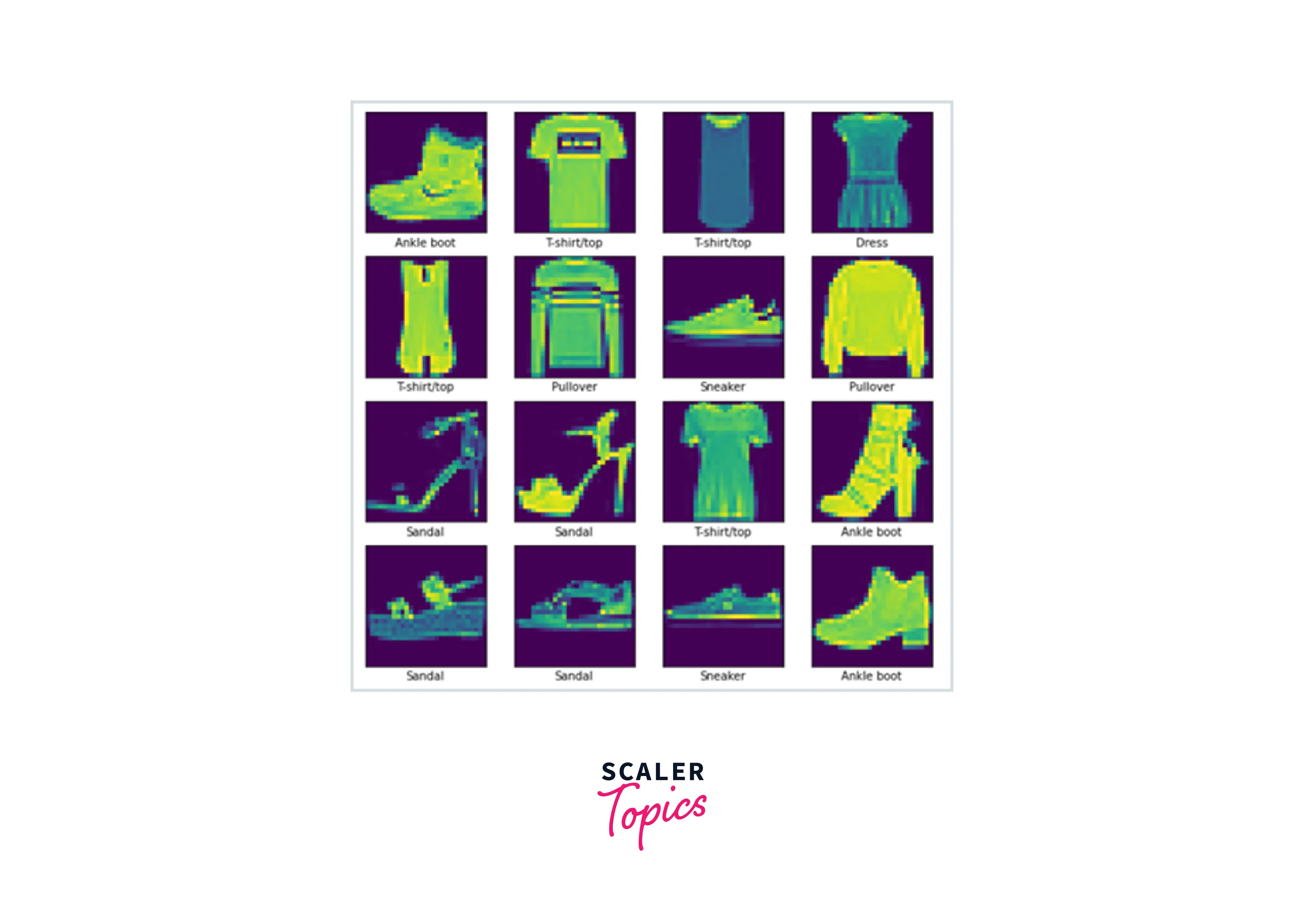
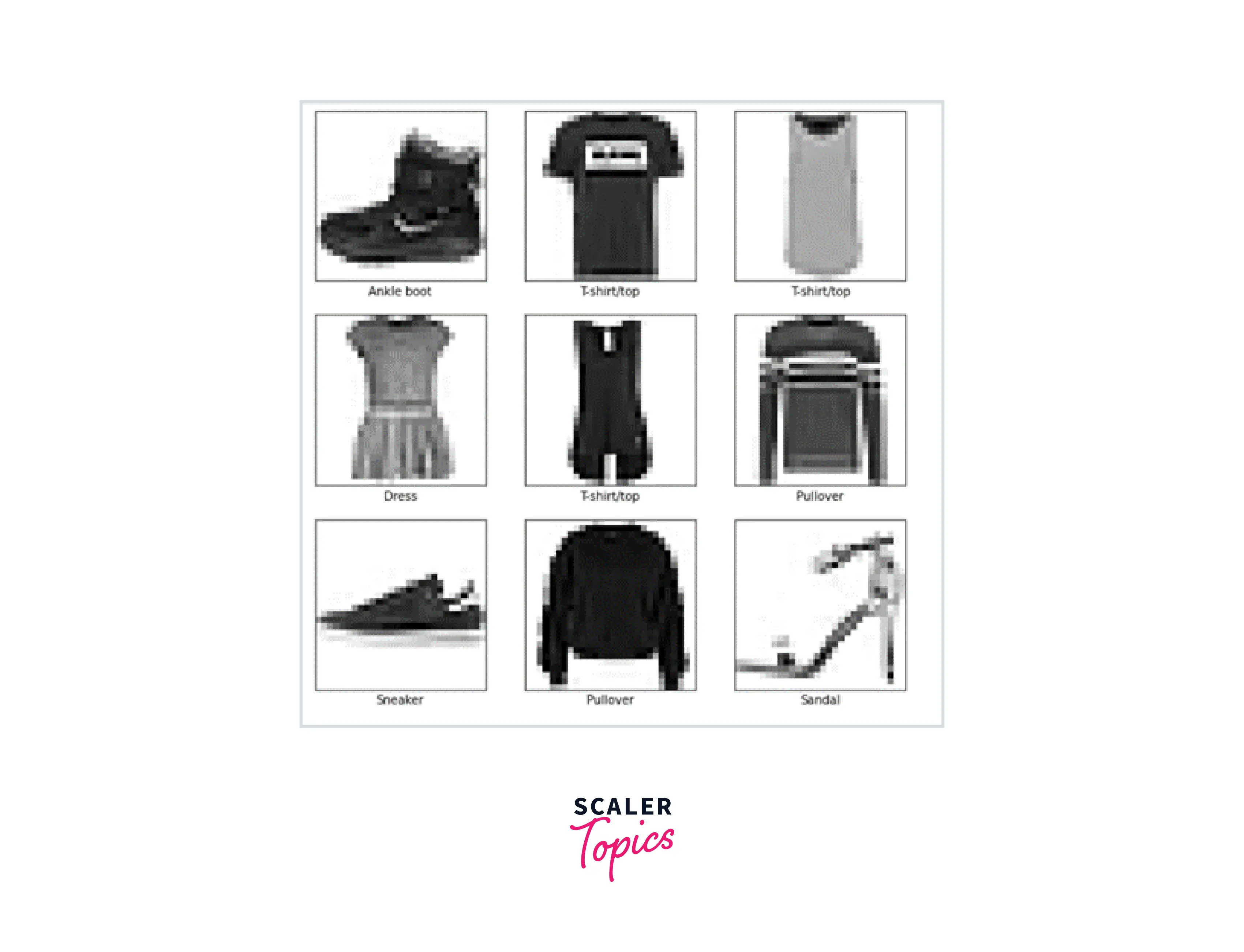
Let us look at the first few images from the training set to confirm that the data is in the appropriate format. We will also display the class name with each image.

Training the Model

In order to create a neural network, the model's layers must be set up as follows:

The above structure is a simple CNN which includes an input layer, hidden layers, and an output layer.

When setting up a neural network, some iterations might be required to decide on the optimum number of layers and the combination of layers to achieve higher accuracy from the model. It is possible to set up this model using a different number of layers and a number of neurons. For example, using 64 or 128 instead of 32 neurons or nodes in the first layers and so on. Note: your accuracy will vary depending on how you set up the model.

Normally, the image features identified by the convolutional layer are reduced in size by the Max Pooling layer, which helps to reduce computations. In other words, the purpose of a Pooling layer is to summarize the image features generated by a convolution layer. Further, we will use the Keras legacy methods of compile() and fit() to train the created CNN. A few more settings such as choosing an optimizer, appropriate loss function, and metrics, are required to make the model ready for training which is added in the compile() command.

Next, we will use the summary() function to see all the parameters and output shapes in every layer of our model.

Output:

To begin training, we will utilize the fit technique, which will fit our model using the training and test data as well as the following inputs:

Output:

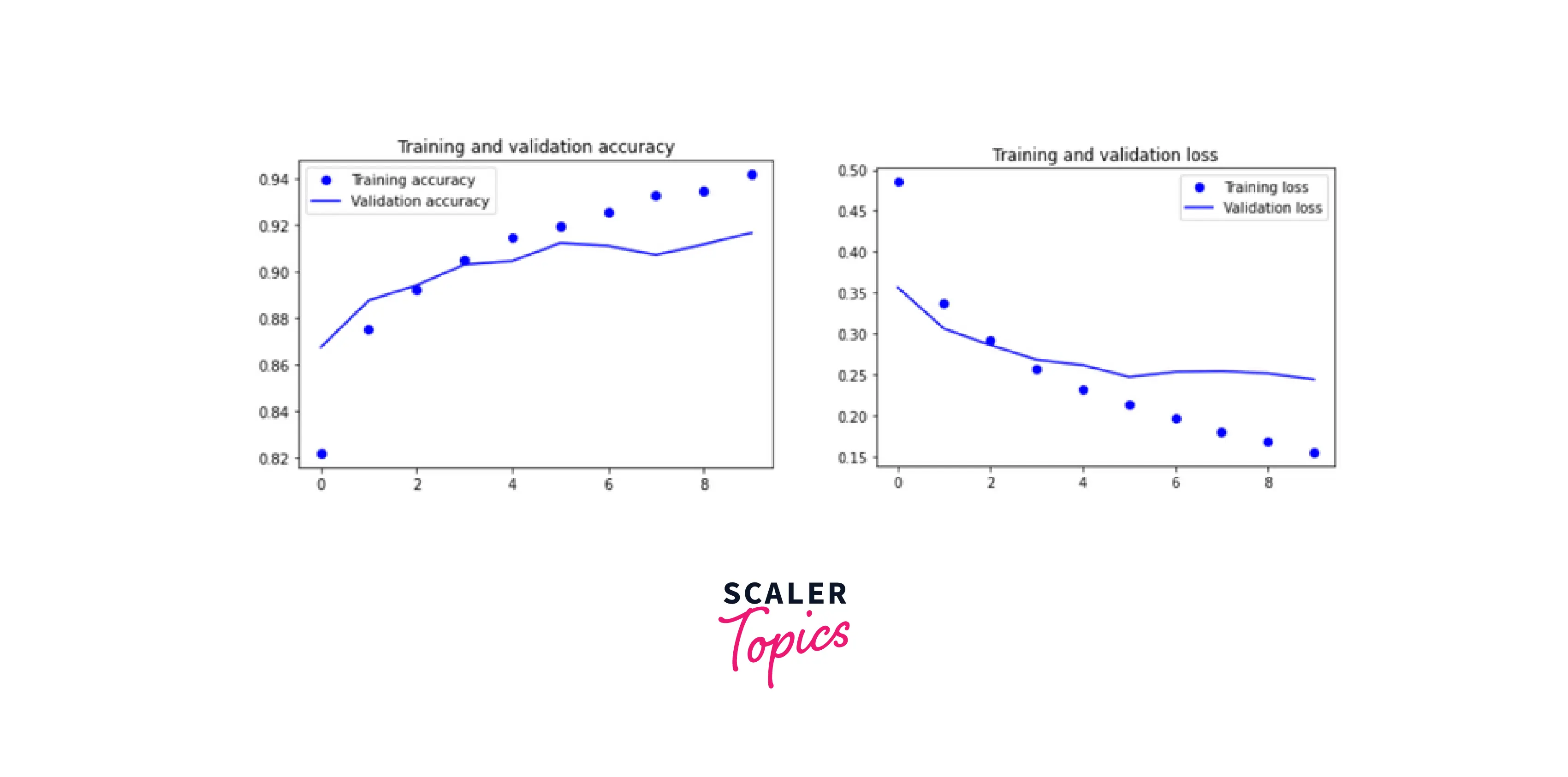
The model training log generated shows the loss and accuracy metrics. This model achieved a good accuracy of about 94% on the training data and 92% on the validation data. Since we had saved the model training history earlier, we can plot the training metrics using any Python visualization library as shown below (optional)-

Performing Inference on Sample Input Image

To make predictions on the test dataset, we use the following command -

Output:

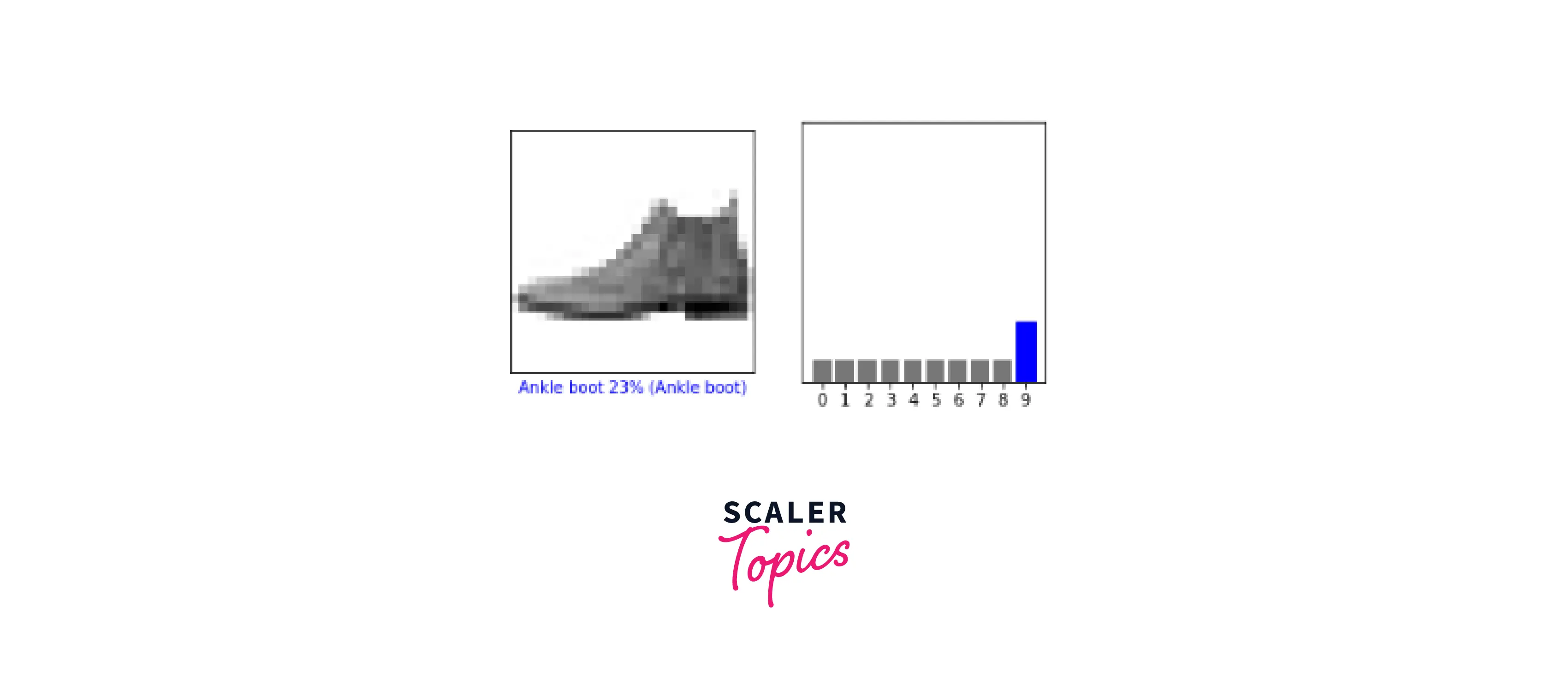
To understand how our trained model makes decisions, we can explore the sample image predictions as -

Where 0 is the first image in the folder.

Output:

These are the ten probabilities or confidence values generated for this image by our model. Identifying the maximum value in the array leads us to category 9 i.e. the 10th label (categories are numbered from 0 to 9) which is an Ankle boot.

Output:

We can also plot the predictions with the image as shown below -

Testing

Once the model training is completed, we can evaluate the model accuracy to see how our trained model performs on the test dataset. We can use the following code -

Output:

The above output indicates that the model achieved 91% accuracy on the test data which means that our model can identify any new images in the clothing and footwear categories accurately.

We can make individual image predictions using -

The above code yields an output of 9 indicating that the image predicted is an Ankle Boot.

What’s Next?

After building this model, we can save it with the existing weights using save() legacy method in Keras and reuse it on newer datasets to make predictions. Alternatively, we can also perform a few iterations for adjusting the layers, adding dropout layers, and regularization to improve the model further. The saved model can also be deployed as a simple web app using tools such as Gradio or Streamlit.