Building a House Pricing Model in Keras

What are We Building?

The Real Estate market is quite dynamic, and house prices continue to vary globally. Major cities often tend to see an appreciation in land and housing prices with inflation. This makes Real Estate pricing an interesting yet challenging problem to solve with Machine Learning.

So, we will build a Keras-Regression model that can accurately predict the sale price of a house based on a given set of features.

Description of Problem Statement

Suppose we have a dataset consisting of house prices in California based on some features of a house like the number of rooms, location coordinates, age of the house, etc. Now, we want to predict the sale price for a house in the same locality with some specific features available in the dataset. It would be interesting to discover the features impacting the sale price.

Pre-requisites

You'll need -

• Good understanding of Regression and Statistics.
• Familiarity with Keras syntax and Deep Learning models in Keras.
• Familiarity with Data Visualization tools such as Matplotlib or Seaborn.

How Are We Going to Build This?

For this, we will require a sample tabular dataset with house features and sale prices of a locality. This dataset can be used to train and build a multi-variable regression model that evaluates the correlation between the features and the target, i.e., the median house values in the local currency. We will employ a neural network to develop this Deep Learning model suitable for a regression task.

Final Output

We will predict house sale prices in the California region where the given 8 numerical properties describe the houses. The target variable MedHouseVal indicates the median house value for California districts and is expressed in hundreds of thousands of dollars ($100,000).

Requirements

To build this Deep Learning regression model, we'll need -

• Libraries such as Pandas, NumPy for processing our dataset, Matplotlib, and Seaborn for Data Visualization.
• The Keras framework for implementing our neural network.
• We would also use Scikit-Learn for outlier detection and scaling our dataset.

Building a House Pricing Model in Keras

Let us begin building an effective sale price prediction model in Keras.

Dataset

Two popular datasets for housing prices are available, i.e. Boston Price Index Dataset and California housing price. Although the popular Boston Price Index Dataset is a built-in dataset in Keras, its use is discouraged due to ethical issues. So, we'll use the California housing price for this lesson instead. This dataset from the StatLib repository can be fetched from the internet using scikit-learn.

Description of Problem Statement

We have to build a Deep Learning regression model in Keras that analyzes multiple features of a house and predicts a sale price for it.

Data Preprocessing

Let us explore the dataset to understand what it includes. We will first import the necessary libraries along with the Keras framework using the following code -

Next, let us import the required dataset and print the column names-

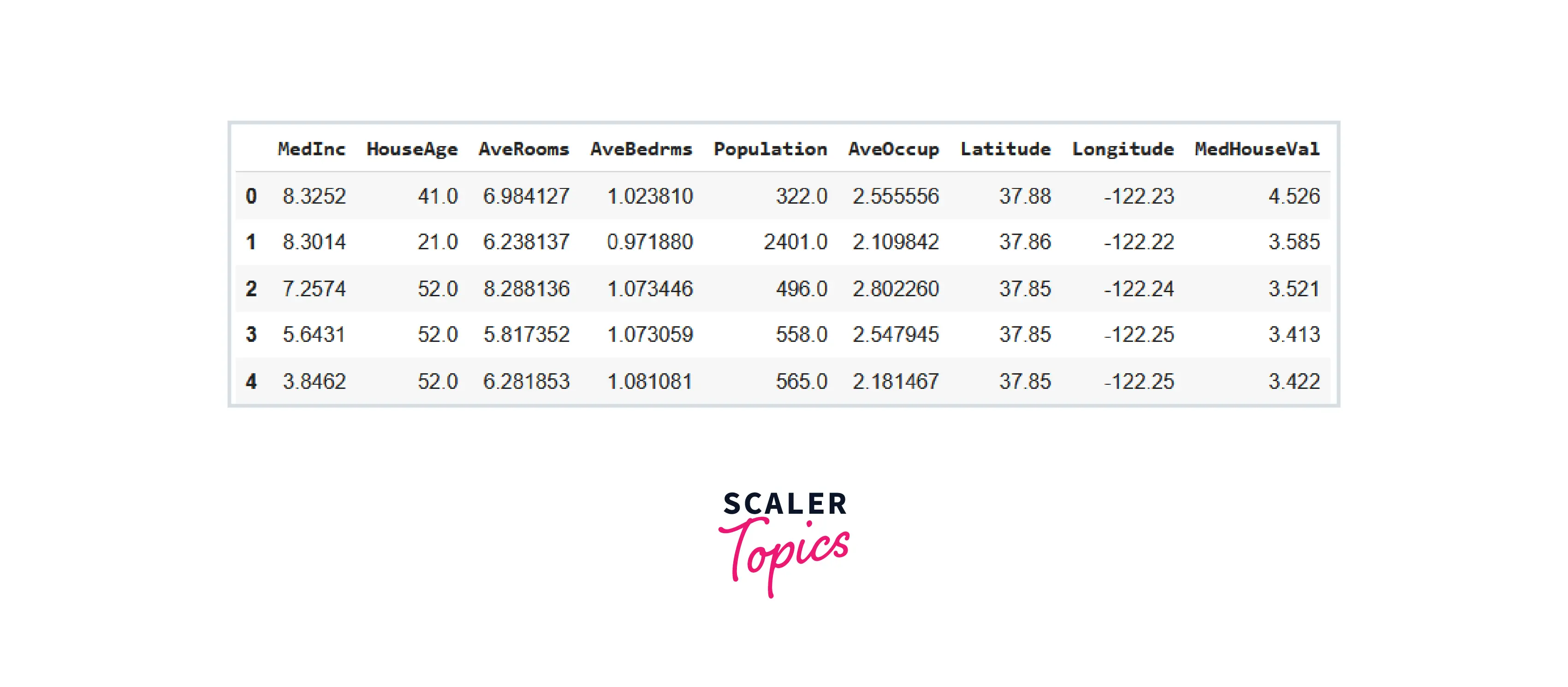
We need to convert the imported dataset into a dataframe using the -

Now, we will check the size of this dataset using the df.shape command.

Brief description of the features

The dataset has 20640 rows. It contains 9 features described as follows:

• MedInc: median income in block group
• HouseAge: median house age in block group
• AveRooms: average number of rooms per household
• AveBedrms: average number of bedrooms per household
• Population: block group population
• AveOccup: average number of household members
• Latitude: block group latitude
• Longitude: block group longitude
• MedHouseVal: median house value for California districts

With the df.info() command, we can understand which data types we will be working with when using this dataset.

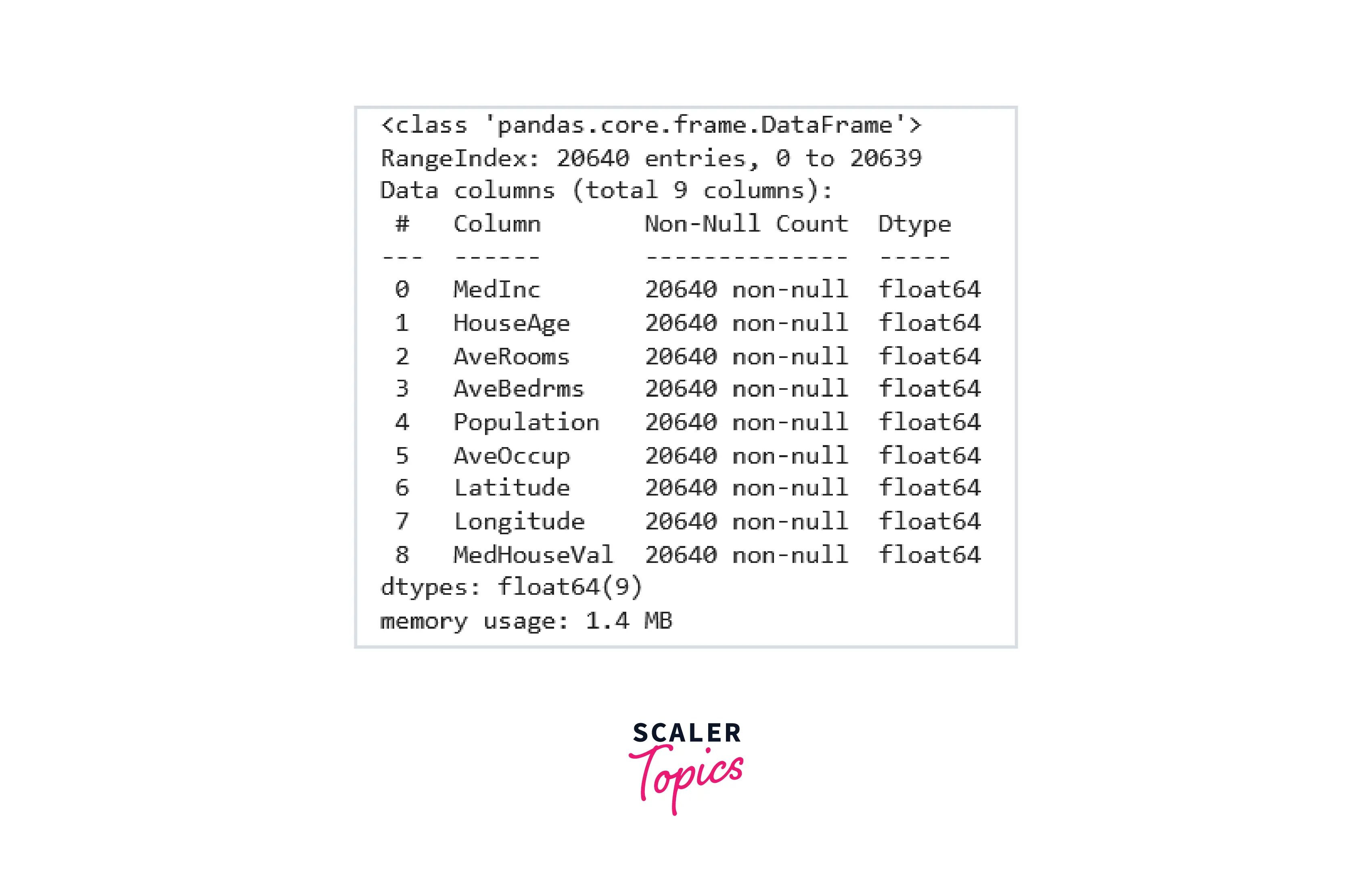
Next, we need to find out if there are any missing entries in the dataset. For this, we will use the following code-

Output:

We’ll perform a short Exploratory Data Analysis (EDA) to check the quality of our dataset, correlation amongst variables and the target, identify any outliers, etc.

First, to explore the distribution of all dataset variables, we can use the df.hist() command in pandas with a bin size of 50. Note that you can use a different number for bin size but the number should not be too high (leads to noise in visualization) or too low (no useful pattern might be visible). The following command displays a grid of multiple histograms, one histogram for each variable.

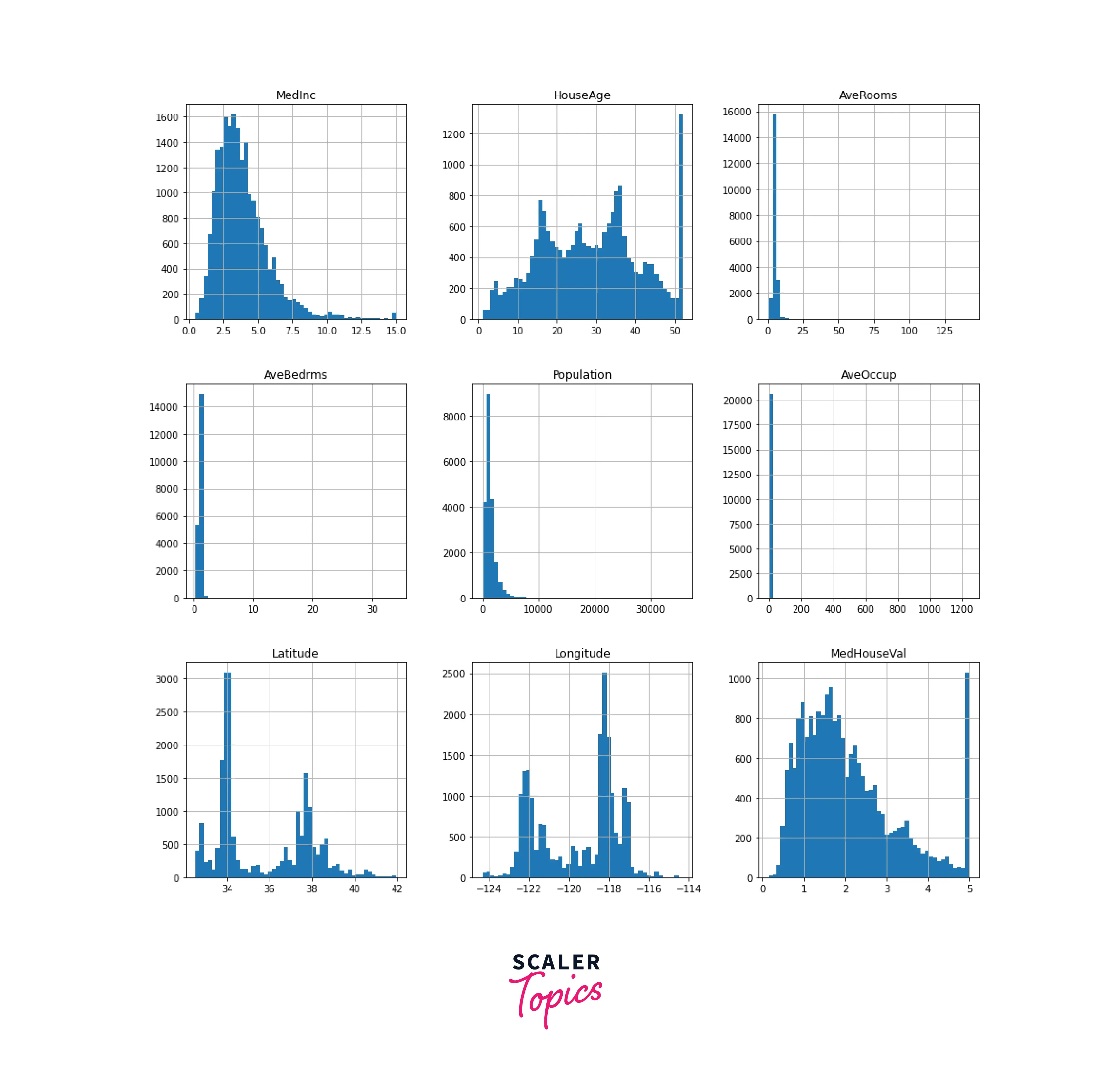
As you can see from the above plots, all the features have different scales, so we need to rescale all the attributes before setting up the model. Besides, we can also spot a few outliers in the dataset. It is possible to extract more information about the data with different plots. In the following plot, we will check the correlation matrix for the dataset.

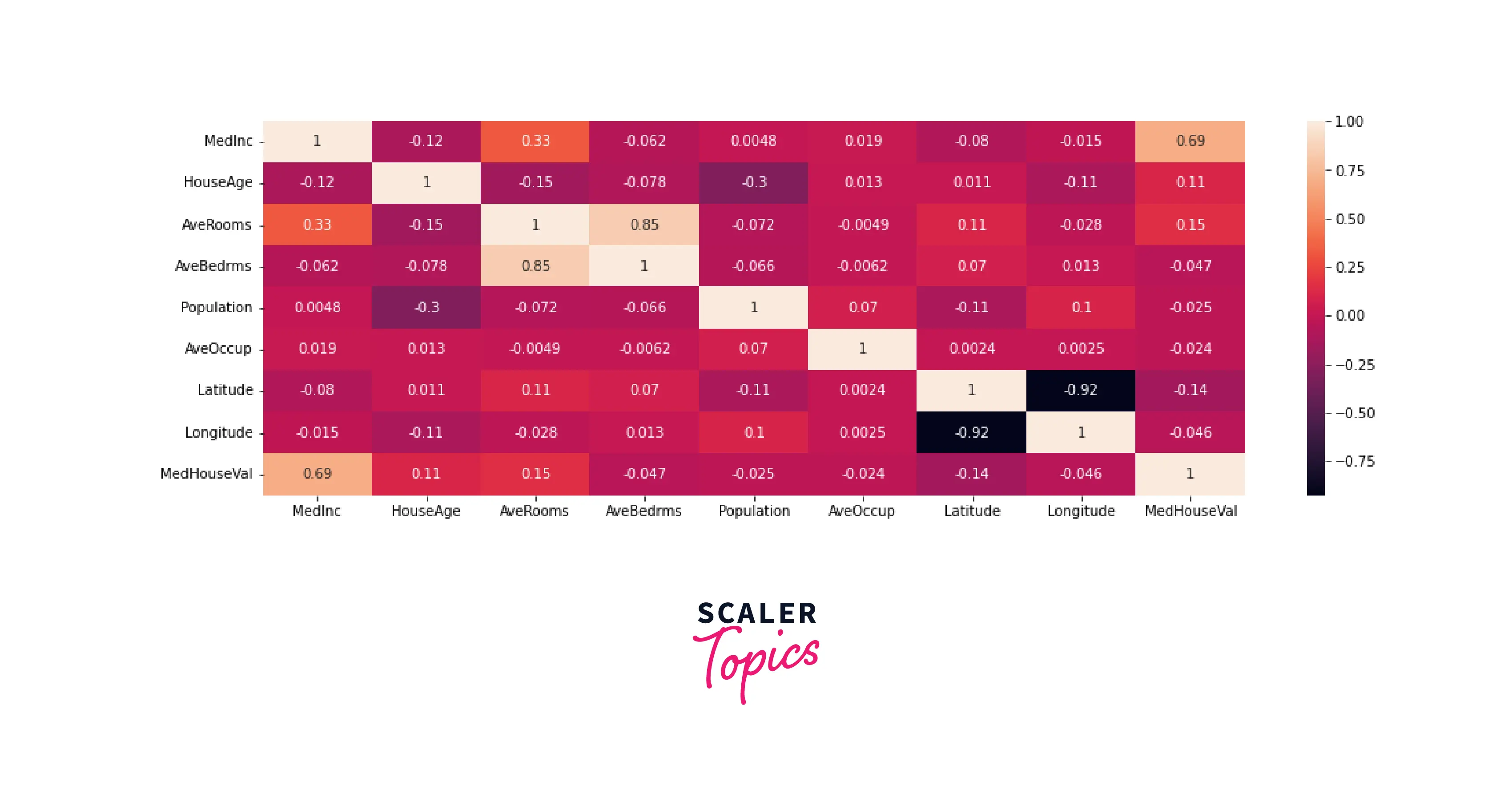
We can see obvious high correlations such as latitude and longitude, AveRooms and AveBedrms as well as MedInc with MedHouseVal.

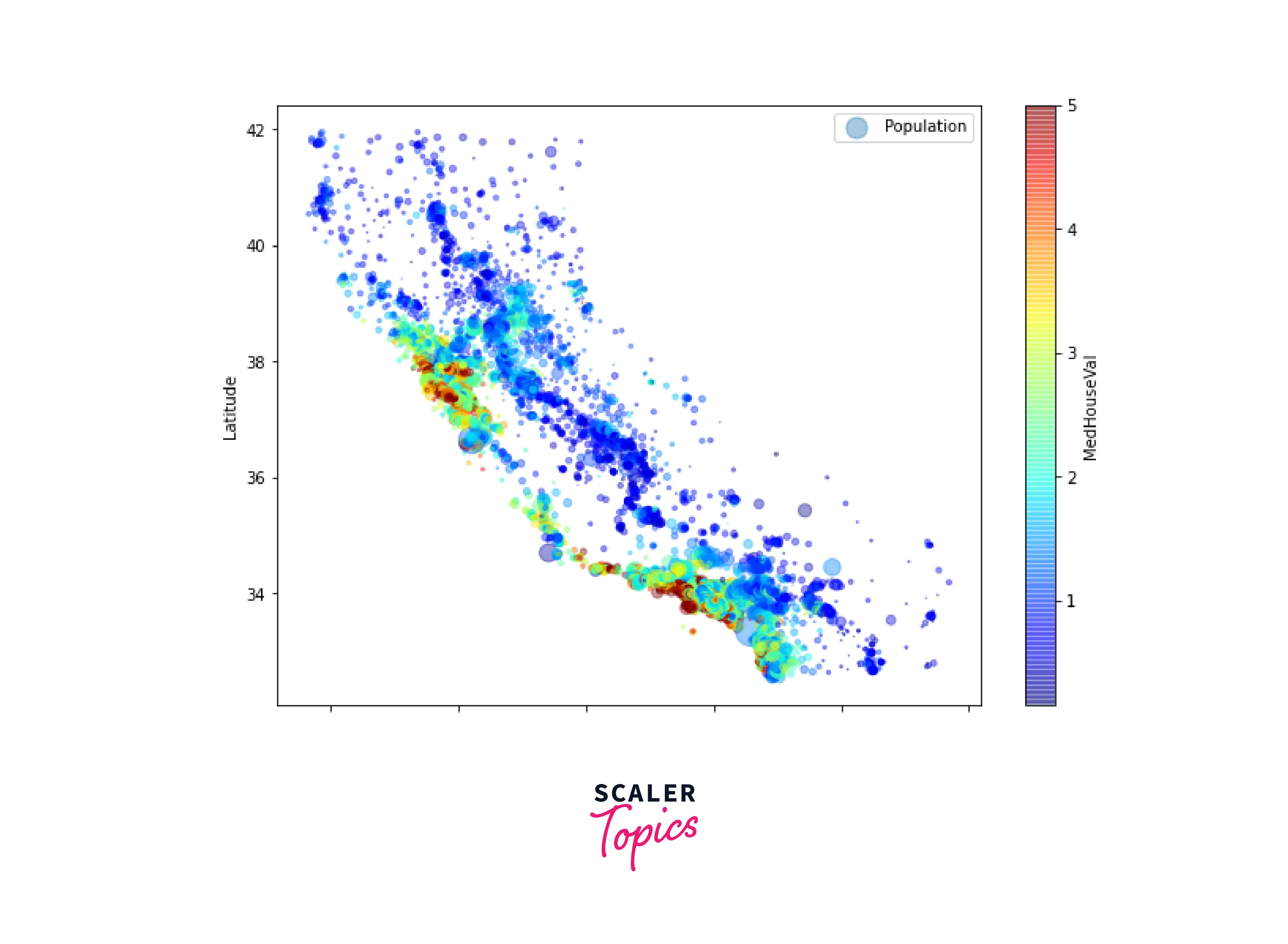
Another interesting plot we can create using the data is a scatterplot for location, population, and median house value. This type of plot can highlight clusters of locations that have either a lower or higher house sale price. To plot this visualization, use the following lines of code -

Let us create an X set (features set or independent variables), and a y set (target or dependent variable) from the dataset.

Now, we will preprocess this data in the next section.

Splitting the dataset

We will split the dataset in an 80:20 ratio using sklearn train_test_split command.

We have split the dataset first and will apply standardization techniques later. You can first apply standardization for this project and then split the dataset. Still, it is essential to remember that in the real world, there are chances of data leakage from the test set into training if you use the latter approach.

Standardization of the Features

Our dataset variables have different scales and units, and hence, these need to be standardized before feeding these to the neural network. The standard scaler command from sklearn will rescale the values between [0,1] for all dataset features. So, we now fit the scaler on our training data, then standardize both the training and test set with the same scaler.

Build the House Price Index Model

As we have already imported the Keras library earlier, it is time to implement the neural network using the Keras Sequential API. For demonstration, we are using three Dense layers in the network with ReLu activation, one Dense output layer with a single value, and choosing the Adam optimizer. You can experiment with a different optimizer, the number of Dense layers and neuron values in these layers, and the activation functions to build your Deep Learning model.

Train and Evaluate the Model

Now, let us train the model using the Keras legacy fit() method. We can also display the model summary to learn more about our model.

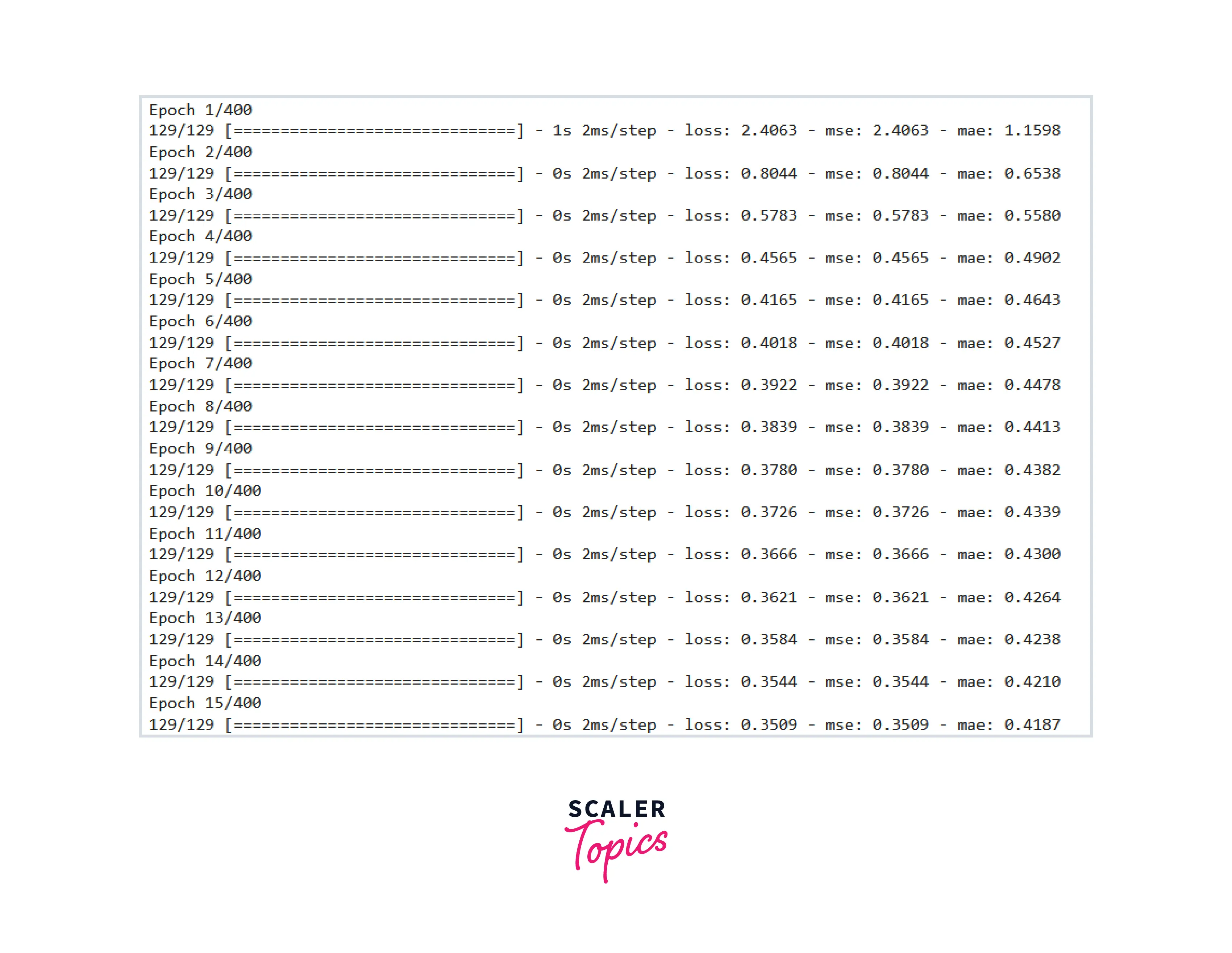
Output

After the training finishes, we will plot the training performance of the model using losses by history callback for Keras .

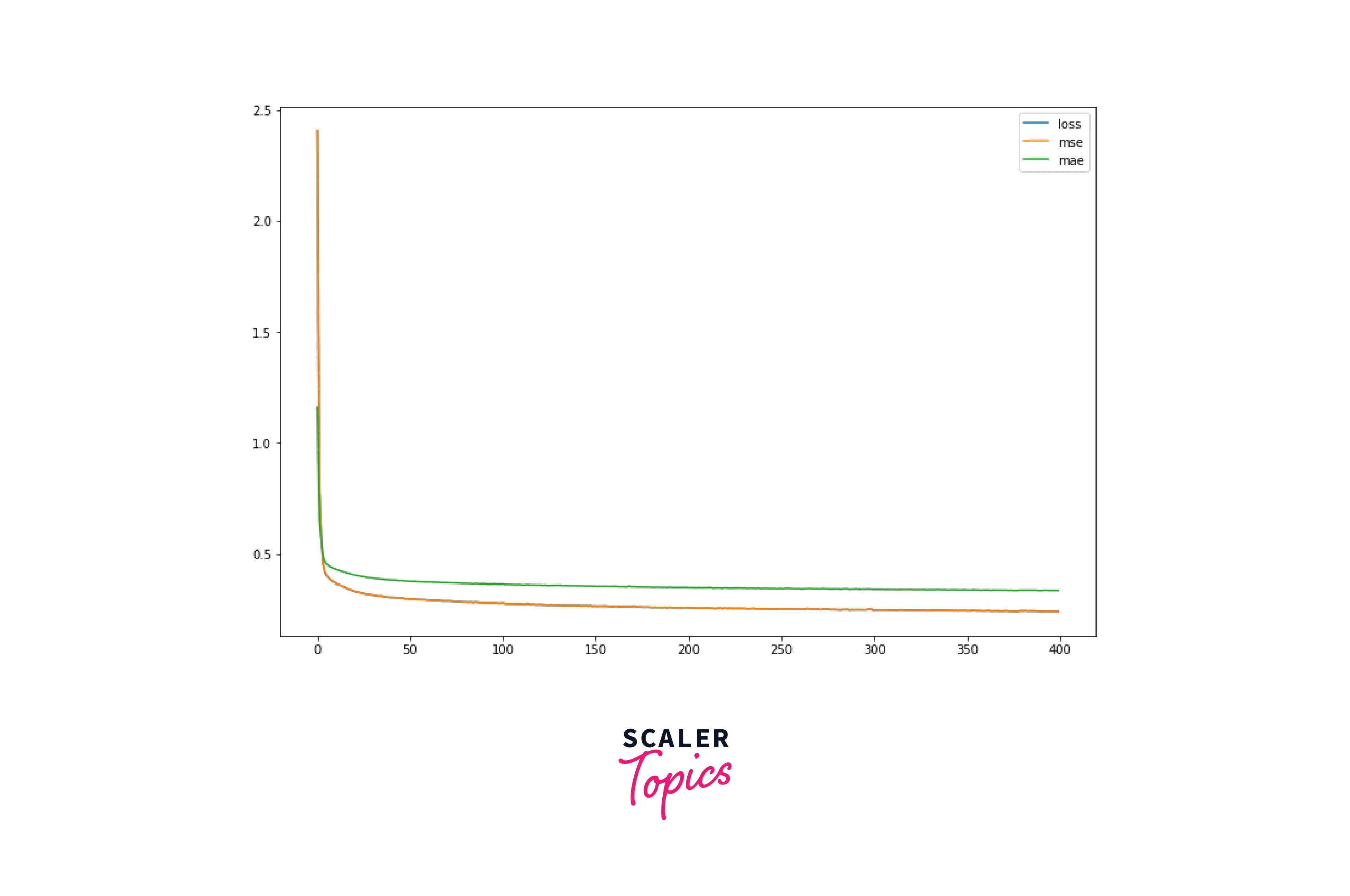
The above plot shows that our model did a good job of reducing the losses, i.e., error in the predicted value over the set 400 epochs. Note if you used a different value of epochs while training the model, your plot might be different.

Evaluate the Test Dataset

We can evaluate the predictions using the -

Output:

Output:

To understand the closeness of predictions with the actual value, we can use sklearn metrics to plot the following -

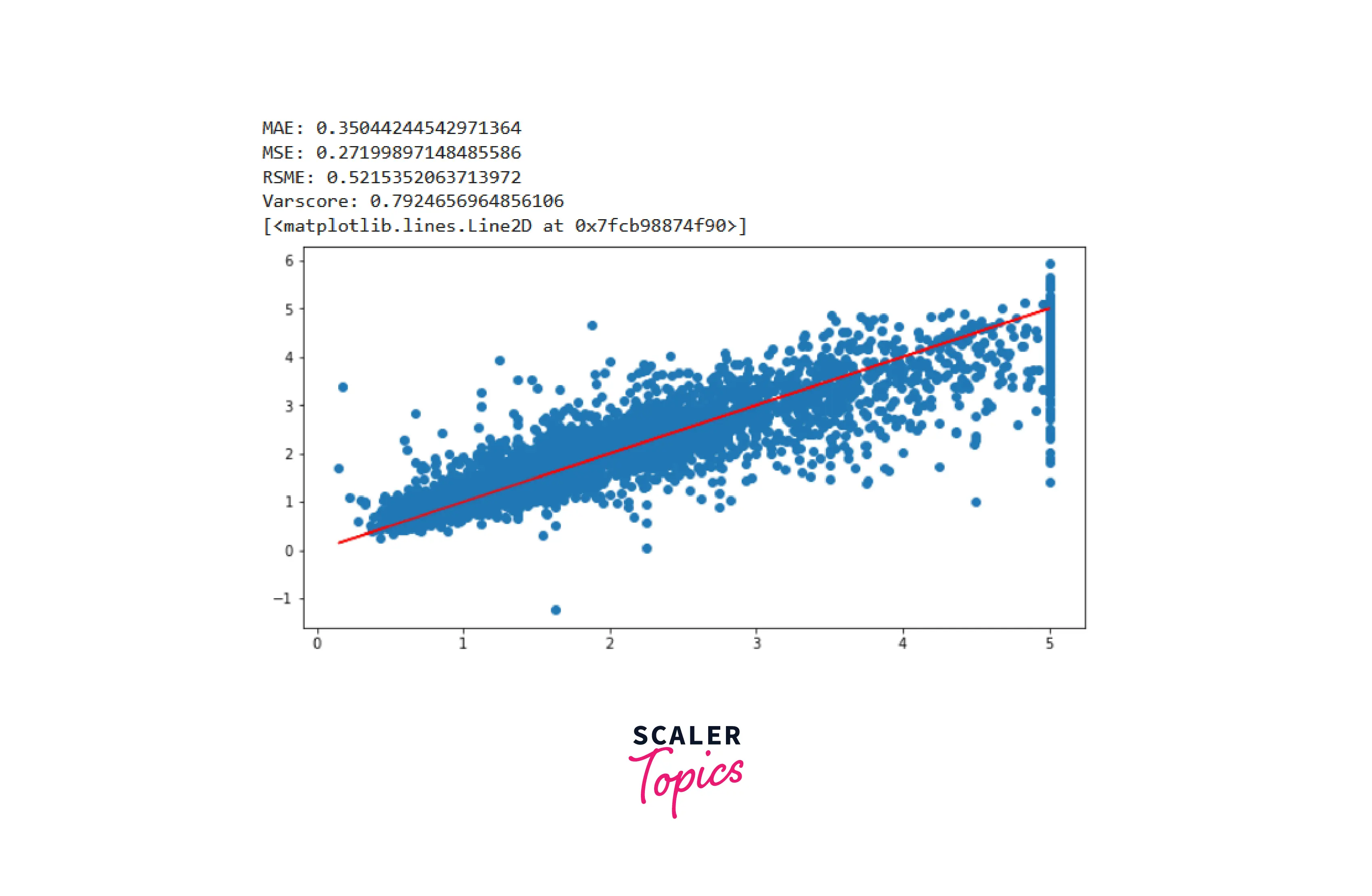
The model did a good job fitting the curve to the provided dataset. However, the outliers can be removed, and the steps could be followed again to improve the model even further.

Testing

We can check the model for a single prediction from the test dataset using the below code -

What’s Next

Our initial trained Keras pricing model has a mean squared error of 23%, which means that, on average, the sale price predictions will be either higher or lower by 23%. The model can be improved further by training for more epochs, iterating the layers and neurons, and handling outliers in the dataset. Feature engineering also might be worth considering, i.e., exploring if we can add more samples and features to this dataset or leverage a relevant image dataset for generating more attributes to fine-tune the model.