Developing and Training a Simple Model in Keras

Introduction

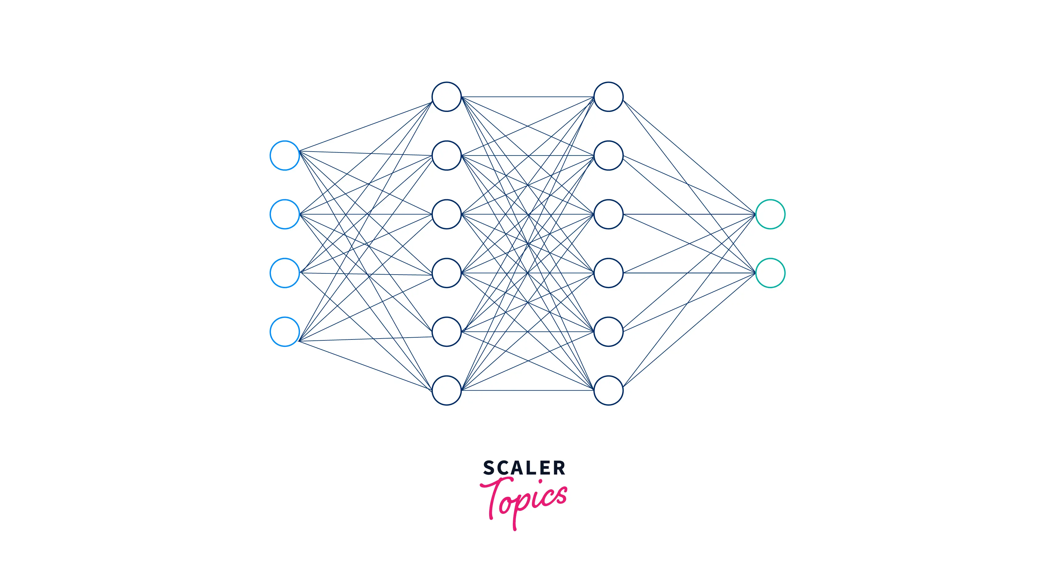
Artificial Intelligence is a field that can be applied in almost all sectors because it requires data to work. Nowadays, every sector is digitized or on the verge of digitization. As a result, the implementation of Artificial Learning is increasing, and there is a huge demand for related professionals in these industries. An artificial intelligence technique called a neural network instructs computers to analyze data in a manner that is modeled after the human brain. Deep learning is a subset of machine learning that employs interconnected neurons or nodes in a layered framework to mimic the human brain.

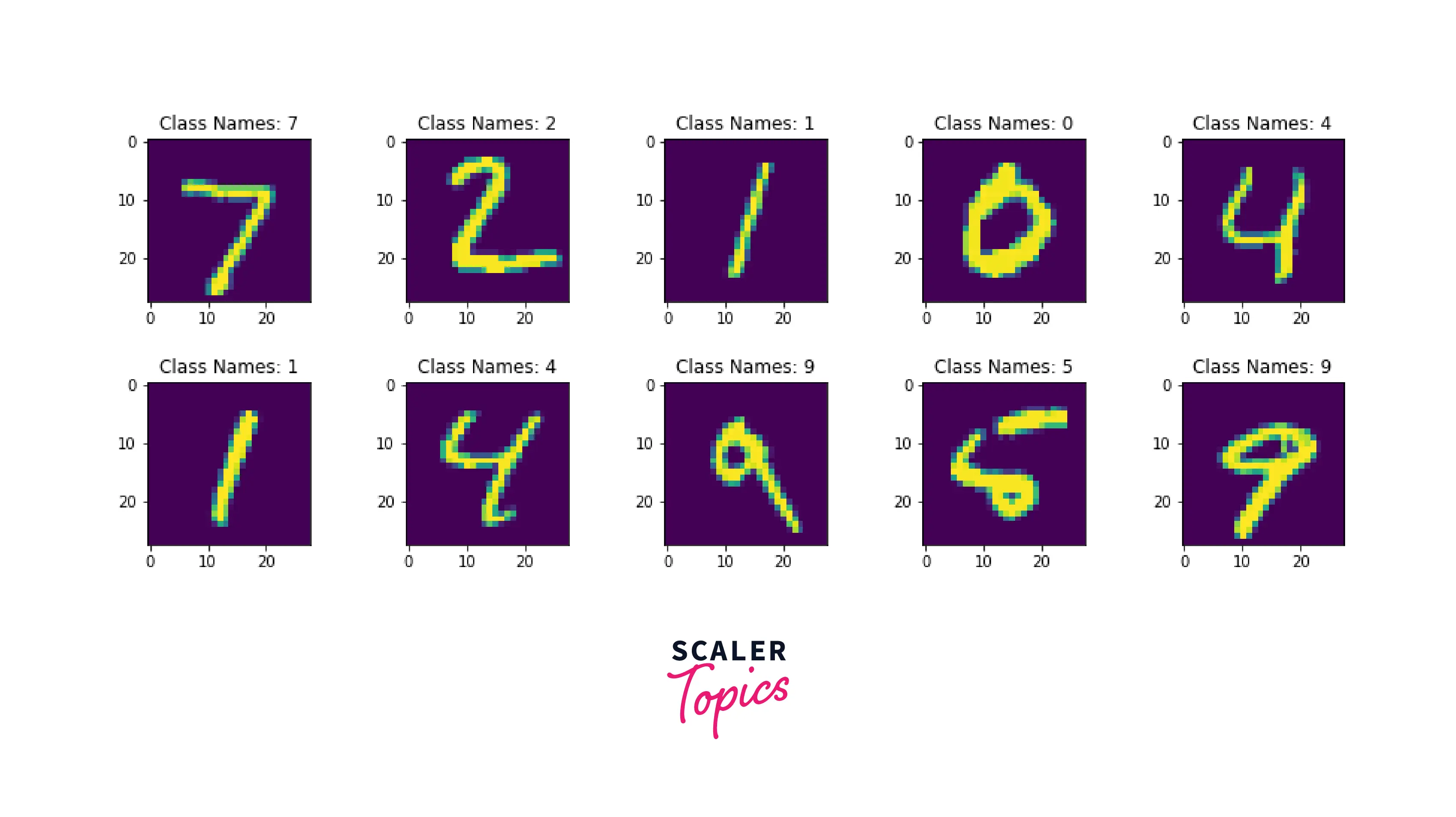
This article will discuss training a simple classifier model based on the MNIST-DIgit Dataset, shown below.

Function of Dense Layer

A dense layer in a neural network is a fully connected layer, where each neuron in the layer is connected to every neuron in the previous layer. The purpose of a dense layer is to learn complex non-linear relationships between the inputs and outputs of the network. Each neuron in a dense layer applies a non-linear activation function to the weighted sum of its inputs, and the layer's output is a set of transformed inputs that can be used as inputs for the next layer. This way, Dense layers can learn and extract features from the input data, allowing the Model to classify or make predictions.

Each neuron in a dense layer takes a set of inputs, performs a dot product of the inputs with a set of weights, and applies an activation function to the result. The output of the dense layer is then passed on to the next layer in the network.

Here is the mathematical representation of this process:

Here, 'input' is the input to the dense layer, 'weight' is the layer's weight matrix, 'bias' is the bias term of the layer, and 'activation' is the activation function applied to the output.

The purpose of the dense layer is to learn complex non-linear relationships between the inputs and outputs of the network. By applying a non-linear activation function, the dense layer can introduce non-linearity into the Model, allowing it to learn and extract features from the input data, providing the Model with the ability to classify or make predictions.

Dense layers are typically used in the middle or toward the end of the network, where they can learn the most complex features and relationships from the input data. The formulae of the metric product are shown below:

X is a matrix with a diagonal of (1, N), and A is a (M x N) matrix. The values inside the matrix are the trained parameters of the earlier layers, and backpropagation can likewise be used to update them. The most popular algorithm for training feedforward neural networks is backpropagation. In a neural network, backpropagation typically calculates the gradient of the loss function relative to the network weights for a single input or output. According to the initial idea, the dense layer will produce an N-dimensional vector as its output. However, we can observe that the vectors' dimension is being reduced. As a result, each neuron in a dense layer is employed to change the vectors' dimension.

Options with Dense Layer

This section will discuss the Keras syntax of the Dense Layer and what options are present in the pre-defined dense layer. We also have the option to create our dense layer with our custom logic by inheriting the layer class and overwriting the respecting class function. The Syntax and option for the dense layer are discussed below Syntax

Parameters

units: Units are one of the most essential and significant aspects of the Keras dense layer that affect how big the dense layer's output is. It must be a positive integer because it specifies the dimensions of the output vector. Type : Integer Activation: In neural networks, the activation function is a function that modifies the neurons' input values. In essence, it gives neural network networks non-linearity so that the networks can understand the relationships between input and output values. The linear activation function will be considered if this Keras layer has no defined activation. Type: Keras function object use_bias utilize the parameter to specify whether or not to employ a bias vector in a dense layer. Use bias is a boolean argument that, if undefined, is set to true. Type : Boolean kernel_initializer: The kernel weights matrix is initialized using this option. The weight matrix, a matrix of weights, is multiplied by the input to extract relevant feature kernels. Type : Matrix bias_initializer: The bias vector is initialized using this parameter. The extra weight sets that correlate to the output layer but don't require any input are known as bias vectors. It is initially set to zeros. Type : vector kernel regularizer: If we initialize any matrix in the kernel initializer, this argument is used to regularize the kernel weight matrix. bias_regularizer: If we initialize any vector in the bias initializer, this argument is utilized to regularize the bias vector. It is initially set to none. activity_regularizer: This parameter is used to regularize the activation function, which we have defined in the activation parameter. It is applied to the output of the layer. By default, it is set as none. kernal_constrained: This parameter applies the constraint function to the kernel weight matrix. It is initially set to none. bias_constraint: This parameter applies the constraint function to the bias vector. By default, it is set to none.

Simple Keras Model

In this part of the article, we will train a simple classification model with Keras. Also, I will explain the legacy functions used to train any Deep Learning (DL) model.

Importing Libraries

The code snippets import the libraries we will use to create the Simple Multi-Class Classifier Model in Keras.

Loading Dataset

Data processing is necessary before supplying information to the neural network. For this exercise, we will use the MNIST-Digit dataset, which contains images of handwritten digits. The dataset is already split into a train set which contains 60000 images, and a test set of 10000 images. It contains ten classes corresponding to the number of digits (from 0 to 9). The classes are mutually exclusive, meaning each image belongs to only one class. The Dataset is commonly used as a benchmark for machine learning and computer vision algorithms and a beginner-friendly dataset for learning image classification techniques. The Dataset may be loaded and transformed into a Numpy array without further splitting because it has already been split into a Test and Training set. As shown in the following code:

Dataset Visualization

Data visualization is one of the most crucial components of any machine learning (ML) or deep learning (DL) project. Here, I will plot the 10 data samples from the training dataset using the code as shown below:

Pre-processing

In this step, I will import the MNIST-Digit Dataset into the tf.data pipeline in this stage. By implementing tf.data Data Input Pipeline, I have constructed two pipelines: test data and train data. The Dataset can be loaded straight from a numpy array using the Dataset from tf.data tensor slices- function. Training models with the help of Data Pipelines is highly recommended in the industry and research because it enables us to directly transfer the Model from the development environment to the production environment. The below code snippets depict the code for loading Train and Test data in the data pipeline for the MNIST-Digit Classifier dataset.

In this section, I created the data pipelines for the MNIST-Digit classifier model in Keras. The arguments for the preprocess function are label and picture. The image pixel is then divided by 255, resulting in a pixel value ranging from 0 to 255. The next step, known as pixel scaling, involves reshaping the images into 28*28*1 dimensions and returning them with their respective labels.

After the Dataset has been preprocessed, the map function is called on the dataset input pipeline, which then calls the preprocess function for each of the samples included in the Dataset. In short, the preprocess function will get one sample at a time from the map function. The Dataset is then shuffled or randomly arranged to rule out any associations between the dataset sample and the dataset sequence. Finally, we implement Prefetch with AUTOTUNE and batch the Dataset into 32 pieces. To ensure no delay while feeding the batches into the Model's training phase, Prefetch always keeps at least one batch ready.

For the Test data pipeline, the same process from the Training data input pipeline is implemented, but we don't shuffle the dataset samples or prefetch any batches.

Model Creation

After preprocessing the Dataset, it’s time to create the Model we will train. For the sake of simplicity, I have constructed a simple Dense Layer Neural Network model.

Sequential explains to Keras that we are sequentially building models, with the output of each layer we define as an input to the layer after it. The first layer of the Model is Flatten Layer with an input shape of 28*28. It will convert the square metric in the 1D vector to make the shape acceptable to the dense layer. The model architecture also constitutes one dense layer with Activation of relu and 128 neurons.

In the MNIST dataset, the images are 28x28 pixels, meaning they have 784 pixels (28x28=784). Therefore, to feed these images into a neural network, they must be transformed into a one-dimensional array of 784 values. This process is called flattening, and it is necessary because most neural networks are designed to process one-dimensional arrays of data.

Flattening the input reduces the dimension of the data, making it easier to process. In the case of MNIST, it is a simple image classification task, so it makes sense to have a flattened image as an input rather than a 2-D array.

The Classification Layer is the bottom layer. This layer has ten neurons since we need to categorize ten different objects. It comprises the activation function known as Softmax, which outputs the probability of the classes linked with the datapoint and has a range between 0-1. The Model's code snippets are displayed below:

Model Summary

In the above section, I have created a simple classification model. It is very important to analyze the model input shape and output shape because it helps us debug the Model if an error occurs. The model summary also shows us the number of parameters the Model has, i.e., trainable and not-trainable parameters.

The below code shows the summary of the Model which we have created above:

The model summary is shown below.

Model Summary displays the following information about the layers:

• Each layer has an output, and the Output Shape column displays the shape of each output. The output from each layer serves as the first layer's input.
• You can see how many parameters can be trained in the "Param #" column.
• At the conclusion, the total number of parameters—which includes both trainable and untrainable parameters—is displayed. All of the layers in this Model can be trained. We won't change the trainability of specific layers to avoid overcomplicating the essay. For your curiosity, Keras allows us to choose which layers to skip training, which makes certain parameters untrainable.

Legacy Methods in Keras

This section will discuss the legacy Keras function/methods widely used to develop and train basic Keras models.

Compile

This section will give us insight into how we can compile any Deep Learning (DL) Model and the components required to compile the Deep Learning (DL) Models.

Optimizer

An optimizer is a method or algorithm used in machine learning and deep learning to update the parameters of a model to minimize a loss function. The main goal of an optimizer is to find the set of parameters that minimize the difference between the predicted output and the true output so that the Model can make more accurate predictions.

Several optimizers are commonly used in AI, each with strengths and weaknesses. Some of the most popular optimizers include:

• Stochastic Gradient Descent (SGD)
• Adam
• RMSprop
• Adagrad
• Adadelta
• Adamax

All of these optimizers have a different approach to updating the weights of the Model, and the choice of optimizer depends on the problem and the Model. For example, the Adam optimizer is a good choice for most cases. This is because it combines the strengths of Adagrad and RMSprop and adapts the learning rate for each parameter.

Loss

In Artificial Intelligence and machine learning, a loss function is a mathematical function that measures the difference or loss between the predicted output of a model and the true output. The goal of training a model is to find the set of parameters that minimize the loss function so that the Model can make more accurate predictions.

Many different types of loss functions can be used depending on the problem and the type of Model. However, some of the most commonly used loss functions include:

• Mean Squared Error (MSE)
• Categorical Cross-Entropy Loss (CCE)
• Hinge Loss
• KL Divergence
• Binary Cross-Entropy Loss (BCE)

For this article, we will use Binary Cross-Entropy Loss (BCE) - which is used for binary classification problems. It measures the difference between the predicted probability of the positive class and the true label. The choice of loss function depends on the problem and the type of Model, and it is an essential part of the training process.

Evaluation Metrics

Every machine learning model uses different metrics to judge its performance on test data. Comparable to Loss Functions, metrics are used to track test data performance. There are various accuracy measurements, including categorical, binary, and accuracy. Probabilistic metrics like binary cross-entropy, categorical cross-entropy, and others are also offered.

We built the Model in the parts above. In this stage, we will compile and train our Model. This component will be used to put our Model together. We must specify the loss function, optimizer, and metrics before compiling the Model. Our Dataset is a multi-label dataset. Hence I used sparse categorical cross entropy as our loss function. In AI and machine learning, a loss function is a mathematical function that measures the difference or "loss" between the predicted output of a model and the true output. The goal of training a model is to find the set of parameters that minimize the loss function so that the Model can make more accurate predictions.

The code snippets for compiling the model are shown below.

Fitting the Dataset

The fit() method trains a model on training data in Keras. It takes several arguments, including the training data, the target data, the number of epochs, and batch size.

The fit() function returns a history object containing the training loss and metrics values for each epoch. This can be used to visualize the training process and determine if the Model is overfitting or underfitting.

The fit() function also accepts additional arguments like validation_data, callbacks, etc. Validation_data is used to monitor the validation loss and metrics during the training process. Callbacks perform certain actions during the training, like saving the Model after certain epochs, early stopping, etc.

In summary, the fit() function is a convenient way to train a model on a given dataset in Keras. It takes the training data, true labels, number of epochs, and batch size as inputs and returns the history object, which can be used to evaluate the training process.

Output

save

In Keras, the save() function is used to save a trained model to a file so that it can be reused later without retraining it. The basic syntax for using the save() function is as follows:

Here, filepath is the file name and path where the Model will be saved. By default, the saved Model includes the architecture of the Model, the Model's weight values, and the Model's training configuration (loss, optimizer).

The save() function also accepts additional arguments like overwrite, include_optimizer and save_format, etc. Overwrite is a boolean value that controls whether to overwrite any existing file at the target location silently. include_optimizer is a boolean value that controls whether to include the optimizer state (if any) when saving the Model. save_format is used to specify the format in which to save the Model.

This saved Model can be later loaded using the load_model() function. The below snippet will save the trained model in .h5 format, which can be used for making predictions.

Evaluate

Once we have trained the Model, we have to evaluate the Model on the Test or Validation set to check whether the Model metric and statistics are acceptable. Generally, we split the Dataset into 3 sets, i.e., Train, Validation, and Test Set. Since I have not split the Dataset into 3 subsets, I will use the Test to predict. The evaluation process is a step in the model-development process that determines whether the model best matches the given problem and data. The Keras model has a function called evaluate that performs the model evaluation. There are three primary arguments:

• Data
• Label
• Verbose (Optional)

The code snippets for model evaluation are shown below:

Output

Predict

Finally, we must use the trained model to predict the real-time dataset. Since we don't have a real-time dataset, we can use the Test dataset for prediction.

We need to use the .predict() method to make the predictions from the trained model. As we get the predictions as a probability for each of the 10 classes, we need to extract the list or array index with the maximum probability for each data point. The code snippets are shown below:

The predicted class is shown below:

There is no difference in the installation of the libraries for GPU or CPU. Even these libraries will use the GPU or CPU based on the availability internally in Keras, but in Pytorch, we have to specify it manually. Below I have shown the GPU and CPU information during the model training step. We have many options to see the CPU or GPU utilization, such as using nvidia commands (watch nvidia-smi), or using the 3rd party libraries such as Wandb.ai or neptune.ai. Below, I have shown the Graphs of the CPU and GPU on Colab. The utilization of the CPU and GPU are shown below: