LR Schedulers in Keras

What Is Learning Rate Scheduling, And Why Is It Important?

Learning Rate Scheduling is a process by which the learning rate of the model is decided and applied while training the Deep Learning (DL) models. It is also a pre-defined schedule or framework that adjusts the Learning Rate (lr) of the Deep Learning Model (DL) as the training progresses. Training Deep Learning (DL) models by SGD - stochastic gradient descent optimization - one of the most difficult optimization tasks. Deep Learning (DL) Models consist of hyperparameters such as the number of neurons, activation function, learning rate, optimizer, loss function, and other parameters. The learning rate is one of the most important hyperparameters which control the degree of weight to be updated in the model by the error. Choosing the learning rate is challenging because if the value is too small, the model will slowly or never converge, i.e., the weight will be updated very slowly. In contrast, if the value is too high, the model may get sub-optimal weights or an unstable training process.

Why Adjust Our Learning Rate (lr) and Use Learning Rate (lr) Schedules?

The learning rate schedule lets you change the learning rate as the training progresses. For example, when we train a Deep Learning (DL) model, the optimizer decides on the direction that gives the largest gradient descent of the loss function.

The learning rate controls the size of the update steps along the gradient (weight updation). This parameter sets the magnitude of the gradient you update. If the learning rate is high, the model converges faster and will solve the problem of local minima, but it may overstep the global minima. On the other hand, a lower learning rate is more receptive to the loss function but may require more epochs to converge and get stuck in local minima. The Learning rate schedule allows you to start training with larger or smaller steps and change the learning rate as the training progresses according to a schedule.

Legacy Learning Rate Schedulers in Keras

Keras Framework has built-in Learning Rate schedulers, which can be invoked by initiating the object of the class. The Learning Rate Scheduler callback in Keras gets executed before the start of the epoch. The learning rate of the model gets initialized by the function we provide in the callback and is updated in the optimizer concerning the current epoch.

Syntax

tf.keras.callbacks.LearningRateScheduler(scheduler)

Arguments

1. schedule: Function, which accepts epoch and current learning rate as an argument and returns new learning rate.

   Type : Function Object

Code Examples

In this section, we will have insight into the Learning Rate (lr) Scheduler callback which is discussed in the above section, Learning Rate (lr) Scheduler callback is an existing pre-defined function. We invoke the class by initiating the object and overriding the existing function, which returns the learning rate for the current epochs and applies it to the optimizer we use in the model.

The below code is an in-depth explanation of the Learning Rate (lr) Scheduler callback in Keras. This article aims to explain the Learning Rate (lr) Scheduler callback in keras implementation so that I will focus on that section of the code snippets.

Step 1. Importing required libraries

The first step is to import the required libraries. Then, the snippets are used to import the required libraries for keras so that the classes and functions can be implemented in our code.

Step 2. Data Loading and Data Preprocessing

For the explanation purpose, I have used the MNIST-Digit dataset, which consists of 60,000 greyscale (composed of only one channel) images of handwritten digits from 0-9. The dataset is split into two sections, i.e., the Train set, which consists of 50,000 images, and the Test set, which consists of 10,000 images. I have also preprocessed the dataset by normalizing and converting the labels into categorical values and reshaping the dataset into 28,28,1 shapes because we will implement the Convolution Neural Network 2D model. First, the dataset is loaded from the Keras MNIST-Digit classification dataset, which is already divided into training and testing sets. Then, the dataset is scaled by dividing each pixel by 255 so that the value of each pixel is between 0 and 255 and then reshaped into 28*28*1. The below code snippets depict the preprocessing steps of the MNIST Digit dataset.

The dataset Shape and Samples are shown below:

Output:

Step 3. Model Creation

Now after preprocessing the dataset, it’s time to create the model, which we will train on the MNIST-Digit Classifier Model. For the sake of simplicity, I have constructed a simple 2D-Convolutional Neural Network model with 1 dense layer with 10 neurons and the activation function of Softmax. Softmax is the activation function that outputs the probability of the class associated with the input. It is ranged between 0 and 1. Since we have 10 classes ( 10 different objects to classify), we have added 10 neurons in the classification layer. The model architecture also constitutes two Convolutional Neural Network Layers with feature maps of 64 and 128 kernel sizes of 3*3, respectively. After each Convolutional Neural Network layer, I have added the max pooling layer with the pooling size of 2*2. The Max pooling layer will extract the maximum value from the feature map patches, and hence the feature maps obtained from the Convolutional Neural Network will be downsampled. A dropout layer with a probability of 0.5 signifies that fifty percent of the neurons in the layer will be deactivated randomly to reduce the chance of overfitting during training time. The below code snippets depict code for creating the model as discussed above.

After model creation, we display the summary in the outputs cell. The model summary consists of the parameter trainable and the non-trainable layer name and output shape of the respective layer. The summary of the created model is shown below:

Output:

Step 4. Legacy Learning Rate (lr) Scheduler Callback

This section will implement the Learning Rate (lr) Scheduler callback. As discussed in the above section, the Learning Rate (lr) Scheduler callback takes one argument, i.e., function object, which returns the learning rate (lr) for the current epoch. This callback is invoked at the start of each epoch.

The below snippet depicts the scheduler function, which returns the learning rate (lr) to the LearningRate (lr) Scheduler callback before the start of each epoch. For demonstration purposes, I check if the epoch number is even. I am returning the Learning Rate (lr) without manipulation, and if the epoch number is odd, I manipulate the Learning Rate and then return it from the function.

The snippets below are the compilation of the learning rate (lr) Scheduler callback object into a list passed to the model.fit as an argument.

Step 5. Compile and Training the Model

In this section, we are going to compile our model. First, we must specify the loss function, optimizer, and metrics to compile the model. I have used categorical_crossentropy as our loss function because our dataset is multilabel. Adam was selected as the optimizer to propagate the error backward. Adam is an extension of the Stochastic Gradient Descent and a combination of the Root Mean Square Propagation (RMSProp) and Adaptive Gradient Algorithm (AdaGrad). For metrics, we have used accuracy for simplicity. You can use any metric based on your problem statement. The below snippets depict the code for model compilation.

After successfully compiling the model, our final step is to train the model with a callback. The dataset will be split into two sets, i.e., training and testing set. The argument validation_split denotes the ratio by which the dataset will be split. In our case, it is 0.1, which signifies that ten percent of the dataset will be used for testing, and the remaining ninety percent will be used for training the model with a batch size of 128. The below snippets depict the code for model training with a legacy callback.

Finally, while executing the training code snippets, we will see the outputs as shown below image which has the printing statement which we included in the callback implementation LearningRate (lr) Scheduler callback and the learning rate (lr) will be applied to the optimizer internally image shown below.

Output:

Linear and Polynomial Learning Rate (lr) Schedules in Keras

In the above section, we have discussed the importance of the Learning Rate (lr) Schedule. In this section, we will discuss the most common Learning Rate Scheduler. While training the Deep Learning (DL) model, errors are propagated backward to optimize the model's weights by the data points/dataset. The backward propagation of the error is done by optimizers such as SGD, Adam, RMSProp, Adadelta, Nadam, Adamax, and many others, which depend upon the data points and the problem statement that we are going to solve using Deep Learning models. Each optimizer can accept Learning Rate (lr) as an argument along with the other parameters. Below we will discuss the types of Learning Rate Schedulers most widely used while training the model. Some of the Learning Rate (lr) schedulers mentioned below are Linear, i.e., linearly decrease lr. Some are Polynomial, i.e., decrease the lr in a polynomial manner, and some can behave as both Linear and Polynomial Learning Rate (lr) Schedulers based on the argument.

Inverse Time Decay/ Step Decay Learning Rate (lr) Scheduler

When we apply the Step Decay Learning Rate to the optimizers, it takes the initial specified value of the Learning Rate (lr) as an argument, drops the value of the initial Learning Rate (lr) based on some formulae pre-defined or according to our problem statement and applies to the epoch. The main focus of Step Decay is that after a specified number of epochs, the current learning rate value will change automatically, i.e., it will decrease, and it is applied in the optimizer. It can speed up / slow the model weights updation based on the epoch number.

Syntax

Arguments

1. initial_learning_rate : The value of the model initial Learning Rate(lr).

   Type: Float

2. decay_step: Step number after which the value of the Learning Rate is to be dropped/decreased.

   Type: Integer

3. decay_rate: Measure by which the value of the Learning Rate is to be dropped/decreased.

   Type: Integer

4. staircase: It indicates whether the Learning Rate (lr) Scheduler will apply the decay as discrete or continuous.

   Type: Boolean

Cosine Decay/ Exponential Decay Learning Rate (lr) Scheduler

Exponential Decay is similar to the concept that initially, the Learning Rate value is high as the training process gradually progresses, i.e., increases the epoch number, and the Learning Rate (lr) gets reduced by the exponential value.

Syntax

Arguments

1. initial_learning_rate : The value of the model initial Learning Rate(lr).

   Type: Float

2. decay_step: Step number after which the value of the Learning Rate is to be dropped/decreased.

   Type: Integer

3. alpha: Minimum Learning Rate value can be applied while training the model.

   Type: Float

Cosine Decay Restarts Learning Rate (lr) Scheduler

Syntax

Arguments

1. initial_learning_rate : The value of the model initial Learning Rate(lr).

   Type: Float

2. first_decay_step: Step number after which the value of the Learning Rate is to be dropped/decreased.

   Type: Integer

3. alpha: Minimum Learning Rate value can be applied while training the model. Fraction of the initial LEarning Rate

   Type: Float

Polynomial Decay Learning Rate (lr) Scheduler

Polynomial Decay is similar to the rest of the Learning Rate (lr) Scheduler concept. In that initially, the Learning Rate value is high as the training process gradually progresses, i.e., increases the epoch number the Learning Rate (lr) gets reduced in a linearly or polynomial manner depending upon the value of the argument. It is a special type of Learning Rate Scheduler that can behave as a Linear and polynomial Learning Rate Scheduler.

Syntax

Arguments

1. initial_learning_rate : The value of the model initial Learning Rate(lr).

   Type: Float

2. decay_step: Step number after which the value of the Learning Rate is to be dropped/decreased.

   Type: Integer

3. end_learning_rate: Minimum end Learning Rate value can be applied while training the model.

   Type: Float

4. power: The power/degree of the Polynomial which will be applied while dropping the Learning Rate. The default value of the argument is 1.0.

   Type: Float

5. cycle: Indication whether the Learning Rate scheduler cycle after the decay step.

   Type: Boolean

Piecewise Constant Decay Learning Rate (lr) Scheduler

Piecewise Constant Decay is the type of Learning Rate Scheduler which accepts the epoch boundary, i.e., the range of the epochs, along with the Learning Rate (lr) and applies the specific Learning Rate by the ranges of epoch specified in the boundary. This scheduler treats epochs of the model as a list and applies the specified Learning Rate(lr) to the model optimizer according to the argument.

Syntax

Arguments

1. boundaries: The epoch boundary i.e., the list of the epoch number up to which the specific value of Learning Rate will be applied.

   Type: List of Integer

2. values: The Learning Rate (lr) values list will be applied to the element boundaries.

Implementing Custom Learning Rate (lr) Scheduler in Keras

Warmup Cosine Learning Rate (lr) Scheduler

Learning Rate (lr) is one of the topics which divides the researchers based on their experiences, journals, and state-of-the-art benchmarks since different optimizers utilize Learning Rate in their way (specified by the algorithm).

Warmup Cosine Learning Rate (lr) Scheduler is the outcome of many research paper analyses on Learning Rate schedulers. When we train any model, and in the initial stages of training, weights are far from the ideal values. If we update the weight by a huge learning rate i.e, we apply overcorrection over corrections. The weights which have been correctly adjusted will be overpowered by the weights which have been over correctly, and the network weight will become unstable. As a result, the initial training phase of the model will be unstable, and the model will take more time for convergence i.e., reaching the global minima.

This is the condition where Learning Rate (lr) plays a very crucial role. We start with a very small value of Learning Rate (lr) close to zero, and as the learning progresses, we increase the Learning Rate by linear or polynomial Learning Rate Scheduler. Other Lear ningRatese Schedules, such as cosine decay and linear reduction, can gradually drop the Learning Rate after attaining the initial rate until the training is complete. Learning Rate warmup is typically the first schedule in a two-schedule program, with the second schedule taking over when the rate reaches the initial Learning Rate (lr) i.e, starting point.

Training Image Classifier with Warmup Learning Rate Scheduler

In this section, we will implement Warmup Cosine LR Scheduler with Keras. The model we will implement is MNIST-digit classification with Convolutional Neural Network (CNN). In this section, we will reuse the blocks of code snippets from the section i.e., importing the libraries, Data Preprocessing, and creating the model.

Step 1. Importing required libraries

The first step is to import the required libraries. The snippets are used to import the required libraries for keras so that the classes and functions can be implemented in our code.

Step 2. Data Loading and Data Preprocessing

For the explanation purpose, I have used the MNIST-Digit dataset, which consists of 60,000 greyscale (composed of only one channel) images of handwritten digits from 0-9. The dataset is split into two sections, i.e., the Train set, which consists of 50,000 images, and the Test set, which consists of 10,000 images. I have also preprocessed the dataset by normalizing and converting the labels into categorical values and reshaping the dataset into a 28,28,1 shape because we will implement the Convolution Neural Network 2D model. The dataset is loaded from the Keras MNIST-Digit dataset, which is already divided into training and testing set. Then, the dataset is scaled by dividing each pixel by 255 so that the value of each pixel is between 0 and 255 and reshaped into 28*28*1. The below code snippets depict the preprocessing steps of the MNIST Digit dataset.

Dataset Shape and Test and Training Samples are shown below:

Output:

Step 3. Model Creation

Now after preprocessing the dataset, it’s time for the creation of the model which we will train. For the sake of simplicity, I have constructed a simple 2D-Convolutional Neural Network model with 1 dense layer with 10 neurons and the activation function of Softmax. Softmax is the activation function that outputs the probability of the class associated with the input. It is ranged between 0 and 1.

Since we have 10 classes (10 different objects to classify), we have added 10 neurons in the classification layer. The model architecture also constitutes two Convolutional Neural Network Layers with feature maps of 64 and 128 kernel sizes of 3*3, respectively. After each Convolutional Neural Network layer, I have added the max pooling layer with the pooling size of 2*2. The Max pooling layer will extract the maximum value from the feature map patches, and hence the feature maps obtained from the Convolutional Neural Network will be downsampled. A dropout layer with a probability of 0.5 signifies that fifty percent of the neurons in the layer will be deactivated randomly to reduce the chance of overfitting during training time. The below code snippets depict code for creating the model as discussed above.

After model creation, we display the summary in the outputs cell. Model summary constitutes parameters trainable or non-trainable, layer name, and output shape of the layer. The summary of the created model is shown below:

Output:

Step 4: Warmup Cosine Decay LR Scheduler

In this section, we will implement the Warmup Cosine Decay Scheduler. As discussed in the above section, this function decides the Learning Rate (lr) based on the arguments global_step,warmup_step, hold, start_lr, and target_lr. The below code snippets depict the implementation in depth.

The below code snippets' main objective is to call the above-create lr_warmup_cosine_decay function and assign the Learning Rate (lr) for the batch. However, now we want to assign the learning rate for the batch of the epoch, so the LearningrateSchuder callback will not work since it is invoked at the beginning of the epoch. Hence, we must inherit the pre-defined callback class from Keras Library and override the on_batch_end and on_batch_start functions.

Function __init__: This function will invoke at the time of the object creation of the WarmupCosineDecay. It will call the constructor and assign the class variable with the values passed by when invoking the object.

Function on_batch_start: This function will invoke at the beginning of the batch and update the Learning Rate (lr) for training the batches. It will initiate the lr_warmup_cosine_decay function with the required argument and update the Learning Rate (lr).

Function on_batch_end: This function will be invoked at the end of the batch. It will extract the value of the Learning Rate from the optimizer and append it to the self.lrs list also it will increase the self.global_step value by 1.

In the code snippets below, we assign the variable warm_up steps with 0.05% of the incremental steps. The value of warm-up steps varies according to the problem statement. Also, we are initiating the object of the Custom Callback class with the required parameters to pass it to the my_callbacks (list).

The snippets below compile all the callback object into an array which is passed to the model.fit as an argument. There are many ways to do it. One of the ways is that we can directly add the individual object of the callbacks which we want to implement while fitting the dataset into the model, but the method which is shown below is the most efficient way to accomplish our task.

Step 5. Compile and Training the Model

In this section, we are going to compile our model. We need to specify the loss function, optimizer, and metrics to compile the model. I have used categorical_crossentropy as our loss function because our dataset is multilabel. Adam was selected as the optimizer to propagate the error backward. Adam is an extension of the Stochastic Gradient Descent and a combination of the Root Mean Square Propagation (RMSProp) and Adaptive Gradient Algorithm (AdaGrad). For metric, we have used accuracy for simplicity you can use any metric based on your problem statement. The below snippets depict the code for model compilation.

After successfully compiling the model, our final step is to train the model with a callback. The dataset will be split into two sets i.e., training and testing sets. The argument validation_split denotes the ratio by which the dataset will be split, in our case, it is 0.1 it signifies that ten percent of the dataset will be used for testing and the remaining ninety percent will be used for training the model with a batch size of 128. The below snippets depict the code for model training.

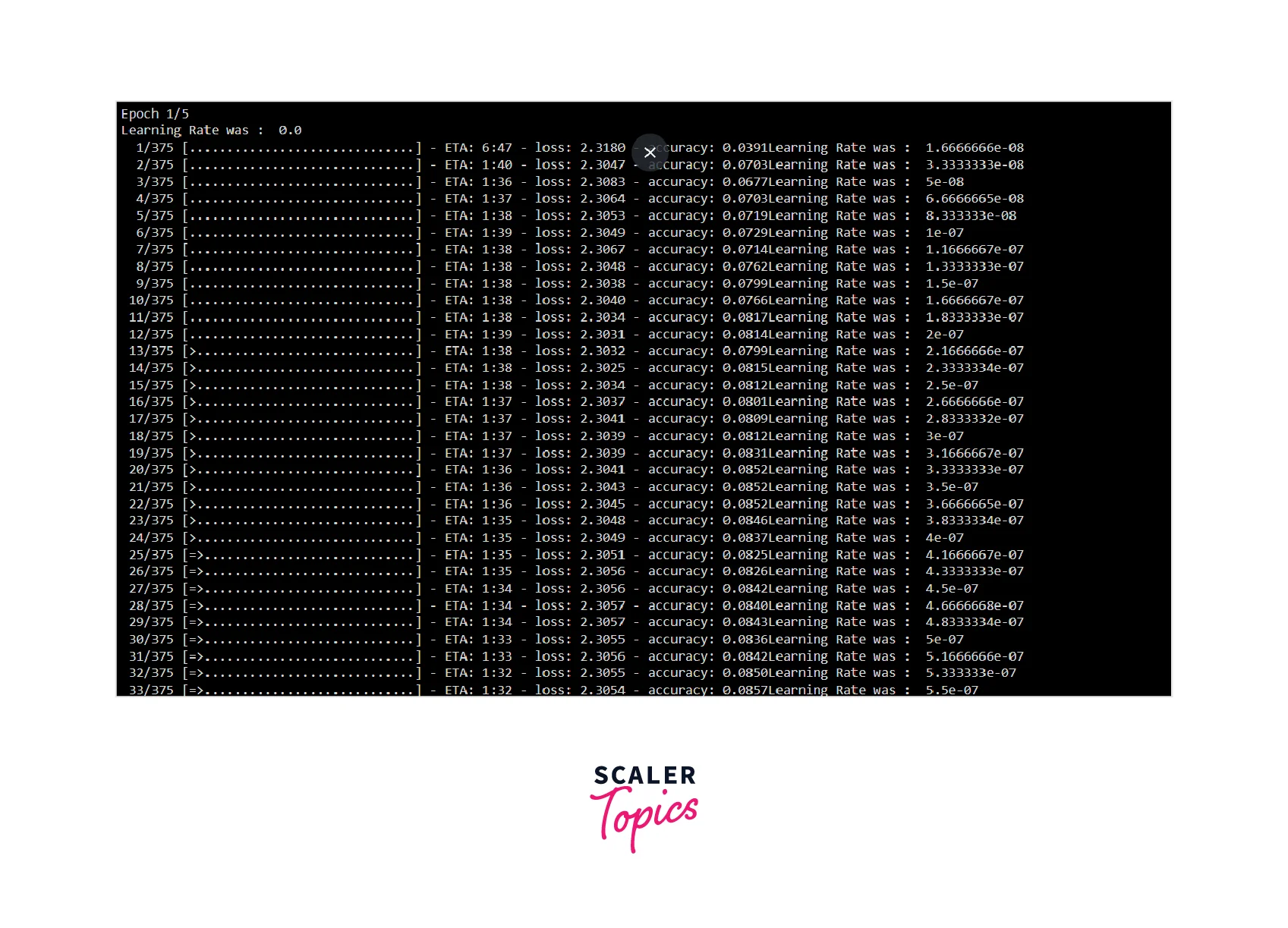
Finally, while executing the training code snippets we will see the outputs as shown below image which has the printing statement which we included in the Warmup Cosine Learning Rate (lr) Scheduler implementation, i.e., it prints the Learning Rate (lr) at the end of the batch.