K-NN Classifier in R Programming
Overview
We can use various machine learning algorithms to predict outcomes based on our data. Some popular machine-learning algorithms include decision trees, random forests, support vector machines, k-Nearest Neighbors from supervised learning techniques and k-means clustering, Apriori from unsupervised learning techniques, etc. We need to choose the right algorithm from several different machine learning algorithms available to us. Our choice of algorithm depends on the nature of our data and the specific problem at hand.
In this article, we will explore the k-Nearest Neighbors classification algorithm. We will discuss how to select the best "K" value and how it impacts our model's efficiency. Also, we will implement the algorithm in R programming and discuss its practical applications to understand its relevance to us.
Introduction to K-NN Classification Algorithm
K-NN is a simple yet powerful supervised machine learning algorithm used for classification and regression tasks. This algorithm's non-parametric nature ensures that it operates without making assumptions about the basic data distribution. It operates on the fundamental principle that data points which are close to each other in a feature space tend to belong to the same class or category. It means that if we have a dataset with multiple classes and are trying to classify a new data point, we can look at the class labels of its nearest neighbors in the feature space to make a prediction.
Example of K-NN Algorithm
To understand the concept of the K-Nearest Neighbors classification algorithm, let us see a simple fruit classification example. Suppose we want to classify fruits into two categories, apricots and almonds, based on two features - weight and diameter. The weight of the fruit is in grams, and the diameter is in millimeters.
Here's what our dataset looks like:
| Weight (grams) | Diameter (mm) | Fruit |
|---|---|---|
| 13 | 11 | Apricot |
| 9 | 8 | Almond |
| 12 | 11 | Apricot |
| 11 | 10 | Almond |
| 10 | 7 | Almond |
| 10 | 6 | Almond |
| 12 | 10 | Almond |
| 13 | 12 | Apricot |
Now, let's say we have a new fruit and want to determine its class (whether it's an apricot or an almond) using K-NN.
| Weight (grams) | Diameter (mm) | Fruit |
|---|---|---|
| 17 | 14 | ? |

At this point, our new fruit entry does not have a class label. To determine its class, we need to calculate the distance from unclassified fruit and fruits in our dataset. There are different methods to calculate the distance such as Euclidean, Manhattan, Hamming distance, etc.
The Euclidean distance is commonly used in KNN algorithm because it works well for most types of data, whereas other methods of measurement like Manhattan or Hamming distances are better for specific types of data such as categorical or grid-like.
Here for our example, we will use the Euclidean distance formula. The Euclidean distance formula, in the context of our fruit classification, can be expressed as:
where:
- X2 represents the weight of the new, unclassified fruit, which is 17 grams.
- X1 represents the weight of a fruit from our existing dataset.
- Y2 represents the diameter of the new, unclassified fruit, which is 14 mm.
- Y1 represents the diameter of a fruit that already exists in our dataset.
Next, we will determine the Euclidean distance between "Unclassified fruit" and each data point in the dataset.
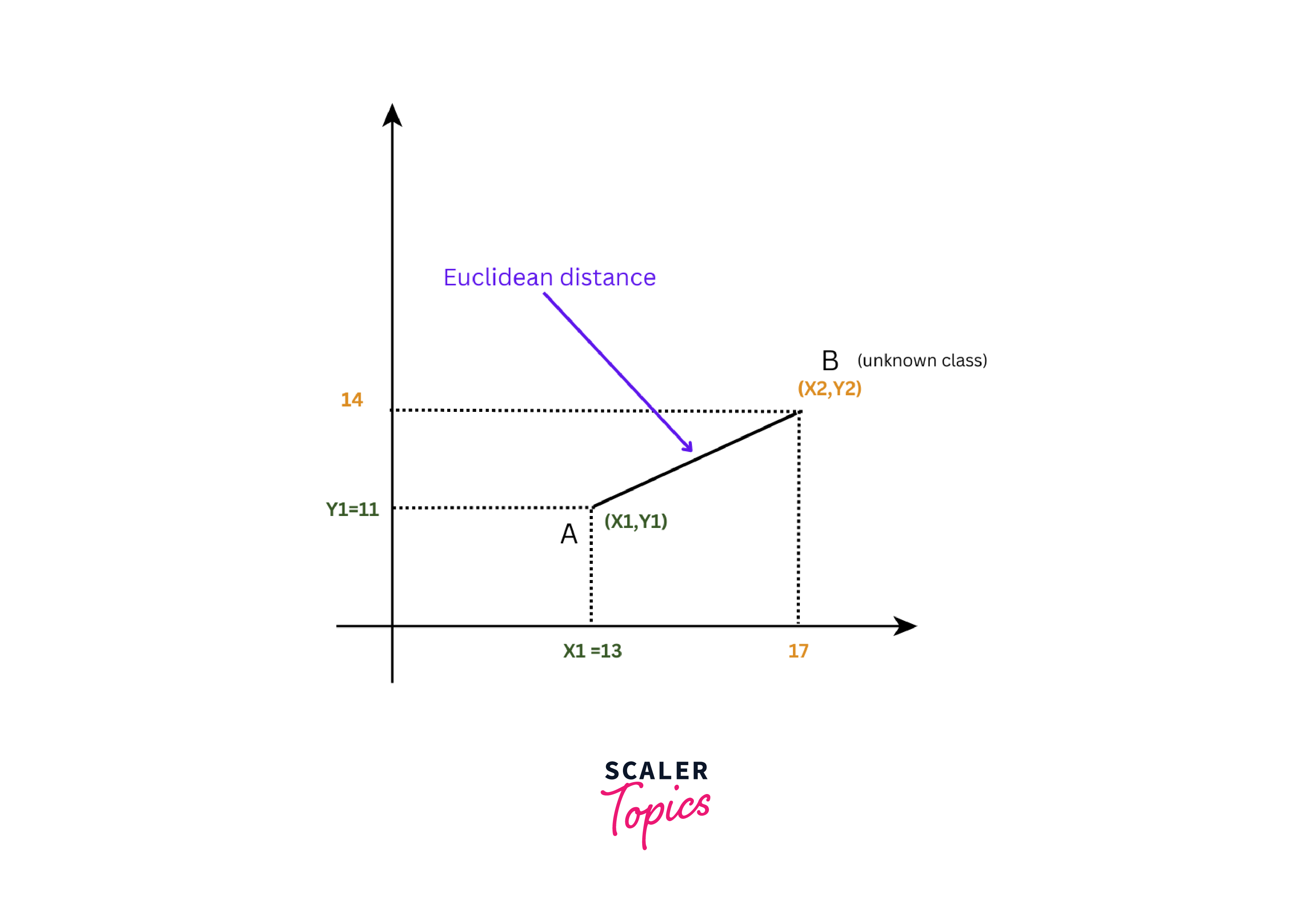
For example, for the first data point (Apricot), X1 is 13, and Y1 is 11. Therefore, the Euclidean distance will be:
Similarly, for the second data point (Almond), X1 is 9, and Y1 is 8. Therefore, the Euclidean distance will be:
We will repeat this calculation for each data point in our dataset. Once we have calculated all the Euclidean distances for all data points, we will arrange the distance values in ascending order as shown below:
| Weight (grams) | Diameter (mm) | Fruit | Euclidean distance |
|---|---|---|---|
| 13 | 12 | Apricot | 4.47 |
| 13 | 11 | Apricot | 5 |
| 12 | 11 | Apricot | 5.83 |
| 12 | 10 | Almond | 6.40 |
| 11 | 10 | Almond | 7.21 |
| 10 | 7 | Almond | 9.89 |
| 9 | 8 | Almond | 10 |
| 10 | 6 | Almond | 10.63 |
Now, we can choose different values of K, representing the number of nearest neighbors we want to consider. For example, if we choose K = 5, we would select the five data points with the shortest Euclidean distances to the unclassified fruit.
| Weight (grams) | Diameter (mm) | Fruit | Euclidean distance |
|---|---|---|---|
| 13 | 12 | Apricot | 4.47 |
| 13 | 11 | Apricot | 5 |
| 12 | 11 | Apricot | 5.83 |
| 12 | 10 | Almond | 6.40 |
| 11 | 10 | Almond | 7.21 |
After identifying the K nearest neighbors, we can count the number of each class (Apricot and Almond) among these neighbors and assign the unclassified fruit to the class with the majority. In this case, since the majority of the five nearest neighbors are Apricots, we would classify the unclassified fruit as an Apricot.
| Weight (grams) | Diameter (mm) | Fruit |
|---|---|---|
| 17 | 14 | Apricot |
Data Preparation/Dataset for K-NN Classification
The foundation of any machine learning project is data preparation, which ensures that the data is in a proper format for both training and evaluation. In this part, we will address the important task of preparing the Sacramento dataset for k-NN classification. It involves several essential steps to convert raw data into a format that can be used successfully for predictive modeling.
The Sacramento dataset contains information about real estate properties in the city of Sacramento. This dataset is commonly used for regression and prediction tasks in machine learning.
Loading the Package and Data
Here, we will use the 'caret' package for this machine learning task. If 'caret' is not already installed, we can easily do so with the following command:
Once the 'caret' package is successfully installed, we can load it and explore the built-in Sacramento dataset, which provides us with information related to properties in the Sacramento area.
The Sacramento dataset consists of various features that describe different aspects of properties. These include the number of bedrooms, bathrooms, square footage, location details, pricing information, etc. Let us print the first few rows of the Sacramento dataset using the following command:
Output:
Creation of Target Variable
We need a categorical target variable to perform a classification task with k-NN. In this case, we will create a binary target variable called 'Price_Category.' Let us estimate a median price value. Next, properties with prices exceeding this median price will be designated as "High." In contrast, those with prices falling below the median will be denoted as "Low."
Output:
Feature Selection
Next, we need to select relevant features from the dataset. For example, we will consider features like the number of bedrooms ('beds'), bathrooms ('baths'), and square footage ('sqft').
Feature Scaling
To ensure that each feature contributes equally to the k-NN algorithm, we will standardize the features using the following code:
Dataset Splitting
To evaluate the performance of our k-NN classifier, we need to split the dataset into a training and a testing set. Further, we train the model using the training set and the testing set will be used to evaluate its accuracy.
Here, we set a random seed for reproducibility. Also, we are using 80% of the data for training and 20% for testing. With these comprehensive data preparation steps, we have transformed the Sacramento dataset into a suitable format for k-NN classification. Now, we will proceed with selecting the optimal 'K' value, building and evaluating the model, and finally making predictions based on property features.
Selecting the Optimal Value of K
We can experiment with different values of K to determine the optimal K for our k-NN classifier. We will evaluate a range of K values to select the optimal K value and choose the one with the highest cross-validation accuracy.
Output:
We used the seq() function to generate a sequence of K values. It starts from 1 and goes up to 20, and increments by 2. These K values represent the number of neighbors the K-NN algorithm will consider when making predictions. Then we applied a loop using the lapply() function that iterates over each K value from the k_values sequence, where:
- A K-NN model is trained using the train() function from the "caret" package for each K value.
- Cross-validation is performed with a trControl argument indicating 10-fold cross-validation. It means the data is split into 10 subsets. Also, it indicates that the model is trained and tested 10 times, with different subsets used for testing each time.
- The tuneGrid parameter is used to specify the K value to test for the current iteration.
- The accuracy is directly stored in the cv_results list, allowing us to compare the performance of different K values.
Let us plot the range of K values and its cross-validation accuracy as shown below:
Output:

Understanding the Impact of K on Model Performance
The value of K in a model can greatly affect its performance. If K is too small, the model may overfit. However, if K is too large, it may result in underfitting. Therefore, it is important to carefully choose the value of K for the specific prediction task.
Cross-validation and Model Selection
Cross-validation is a way to check if a model can make good predictions on new data it hasn't seen before. Now, let us identify the best K value using the following code:
Output:
Handling Even vs. Odd Values of K
In binary classification, choosing an odd value for the K parameter in K-Nearest Neighbors (K-NN) algorithms is a good idea. With an odd K value, there is no chance of having an equal number of nearest neighbours from each class, reducing the possibility of unclear predictions. For example, if K is 15, there is no possibility of a tie between the number of "High" and "Low" neighbours.
Implementing K-NN Classification in R
Finally, we make predictions using the test data and evaluate the model's performance. We will evaluate the accuracy, precision, and recall and create a confusion matrix for our model. All these metrics help us understand how well our model -
- Correctly classifies data (accuracy),
- Identifies true positive predictions (precision),
- And captures all relevant positive cases (recall).
Additionally, a confusion matrix is a chart that graphically shows how well a model makes correct and incorrect predictions, helping us see how good or bad the model is at classifying things.
Output:
Here, we got an accuracy of 0.7891, which means that approximately 78.9% of the observations were correctly classified. The precision, which is the proportion of true positive results among the total number of positive results, is 0.7647. Also, the recall for the "High" class is 0.8387, which means that approximately 83.9% of all "High" observations were correctly classified. Overall, these results tell us that the kNN classifier performed well in classifying observations into "High" and "Low" classes.
Advantages and Disadvantages of K-NN Classifier Algorithm
The k-nearest Neighbors (k-NN) algorithm has several advantages. Some of them are:
- K-NN is a simple and easy-to-understand algorithm.
- K-NN makes no assumptions about the underlying data distribution, making it suitable for a wide range of applications.
- K-NN algorithm can be used for both regression and classification tasks.
However, there are some disadvantages also. They are:
- The K value and distance between data points can greatly affect the performance. Choosing the right values for these two is important, but sometimes this makes it less reliable.
- K-NN can prove to be computationally expensive for large datasets, as it requires calculating the distance between each observation and all other observations in the dataset.
- K-NN may not perform well on high-dimensional data due to the curse of dimensionality, where the distance between observations becomes less meaningful as the number of dimensions increases.
Applications/Use Cases of K-NN Algorithm
The k-Nearest Neighbors (K-NN) algorithm has a wide range of applications. Some of these include:
- Recommender systems:
K-NN can be used to recommend items/products to users based on their similarity to other users. - Anomaly detection:
K-NN can be used to detect anomalies by finding the k-nearest neighbors and determining if the new observation is an outlier. - Medical diagnosis:
K-NN can be used to diagnose medical conditions by finding the k-nearest neighbours and using their labels to make a prediction.
Conclusion
In conclusion:
- K-Nearest Neighbors (K-NN) in R uses the principle that data points that are close to each other belong to the same category.
- Effective data preparation, including scaling and handling missing values, is essential before applying K-NN.
- If K is set too low, the model may overfit. On the other hand, if K is too large, underfitting can happen. Hence, selecting the appropriate K value and evaluating the model using different metrics is necessary.