R Linear Regression

What is a Linear Regression?

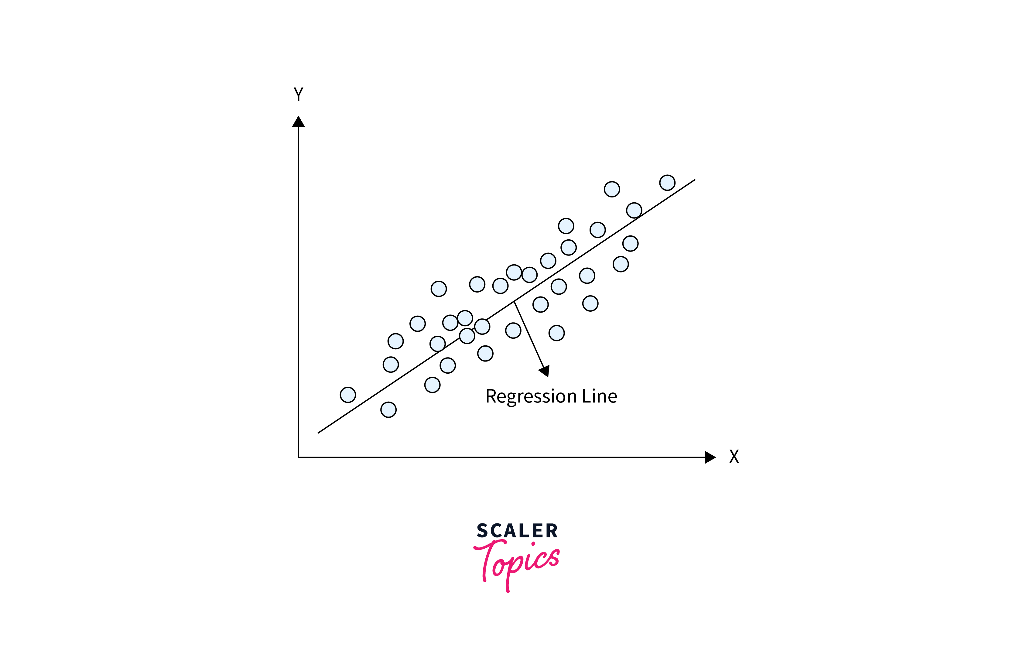
Linear regression is a statistical technique for modeling the relationship between a dependent (y) and an independent variable (x) by fitting a linear equation to the observed data.

It can be expressed mathematically as:

y = β₀ + β₁x + ε

Where:

• y is the dependent variable, i.e., the target we are trying to predict.
• x is the independent variable that influences the dependent variable.
• β₀ is the line intercept.
• β₁ is the linear regression coefficient.
• ε is the error term, representing the residual differences between the predicted and observed values.

Linear regression primarily aims to find the coefficient values that best fit the data and make accurate predictions for new data. It can be done by reducing the sum of squared errors (residuals) between predicted and actual values in the training data.

Once the model is trained, we can use it to predict outcomes for new data by using the values of the independent variables in the linear equation.

Steps to Create a Linear Regression in R

To study the steps involved in performing a linear regression in R, let's consider a simple example of predicting a person's salary based on his or her years of experience. To do this, we need to establish the relationship between the salary of an individual and the years of experience.

Here are the steps:

• In the first step, we will collect a sample of observations of years of experience and the corresponding salaries of individuals.
• Next, we will create a relationship model using the lm() function in R, where we will model salaries as the dependent variable and years of experience as the independent variable.
• After fitting the model, we will find the coefficients representing the relationship between salaries and years of experience. Also, we will create a mathematical equation for predicting salaries using these coefficients.
• Further, to evaluate the quality of the model and understand the average prediction error, we will use the summary() function to obtain the summary of the relationship model. It will give us important statistical metrics about the model's performance.
• Finally, we will use the predict() function to predict the salary on unseen data.

First, let us create a simple employee salary dataset with employee salaries ($) and years of experience they got.

Output:

lm() Function

The lm() function in R is used to fit linear regression models.

Syntax

The basic syntax of the lm() function is as follows:

Here the formula parameter specifies the formula for the linear regression model, and the data parameter specifies the data frame containing the variables used in the formula.

Create a Relationship Model and Get the Coefficients

Now we will use the lm() function with the employee_data data frame that we have created earlier to create a linear regression model relating "salary" (dependent variable) to "experience" (independent variable):

Output:

As the output shows, the experience coefficient is 5697 which means that for each one-year increase in experience, an employee's salary is likely to increase by about $5,697.

Therefore, our linear regression model can be represented as:

Get a Summary of the Relationship

To obtain a summary of the regression model, we will use the summary() function on the model as shown below:

Output:

The summary output includes important data and metrics such as:

• Residuals:
  The residuals represent the differences between the observed and predicted salaries from the regression model. The values range from -2739.4 to 1654.5, with a mean close to zero.
• Coefficients:
  The estimated coefficients for each predictor variable. In this case, the coefficient for "experience" represents the change in salary per unit increase in experience.
• Intercept:
  The intercept term represents the estimated salary when the experience is zero. In this case, the estimated salary is 16466.7.
• Experience:
  The coefficient for "experience" is 5697.0. It indicates that, on average, each additional year of experience is associated with an increase of $5697.0 in salary.
• Residual Standard Error:
  This measures the average distance between the observed salaries and the predicted salaries by the model. In this case, it is approximately 1804, which indicates that the typical prediction error of the model is around $1804.
• Multiple R-squared:
  The multiple R-squared ($R^2$) is a measure of how well the independent variable (experience) explains the variance in the dependent variable (salary). It ranges from 0 to 1; in this case, it is 0.9904. Approximately 99.04% of the salary variability can be explained by the linear relationship with experience.
• Adjusted R-squared:
  The adjusted R-squared adjusts the multiple R-squared for the number of predictor variables in the model. It penalizes the addition of irrelevant predictors. In this case, it is 0.9892, which is very close to the multiple R-squared value.
• F-statistic:
  The F-statistic tests the overall significance of the model. It assesses whether the relationship between experience and salary is statistically significant. In this case, the F-statistic is 823.1 with a very low p-value of 2.357e-09, indicating that the model is significant.

predict() Function

The predict() function in R is used to make predictions based on the linear regression model.

Syntax

The basic syntax of the predict() function is as follows:

Here the model parameter is the linear regression model object created earlier using the lm() function. Also, the newdata parameter specifies the data frame containing the new person's relevant independent variables for which we want to make predictions.

Predict the Salary of New Persons

Here we will create a new data frame called new_data containing the "experience" values for new persons, and now we will predict their salaries using the previously trained model.

Output:

Regression Plotting

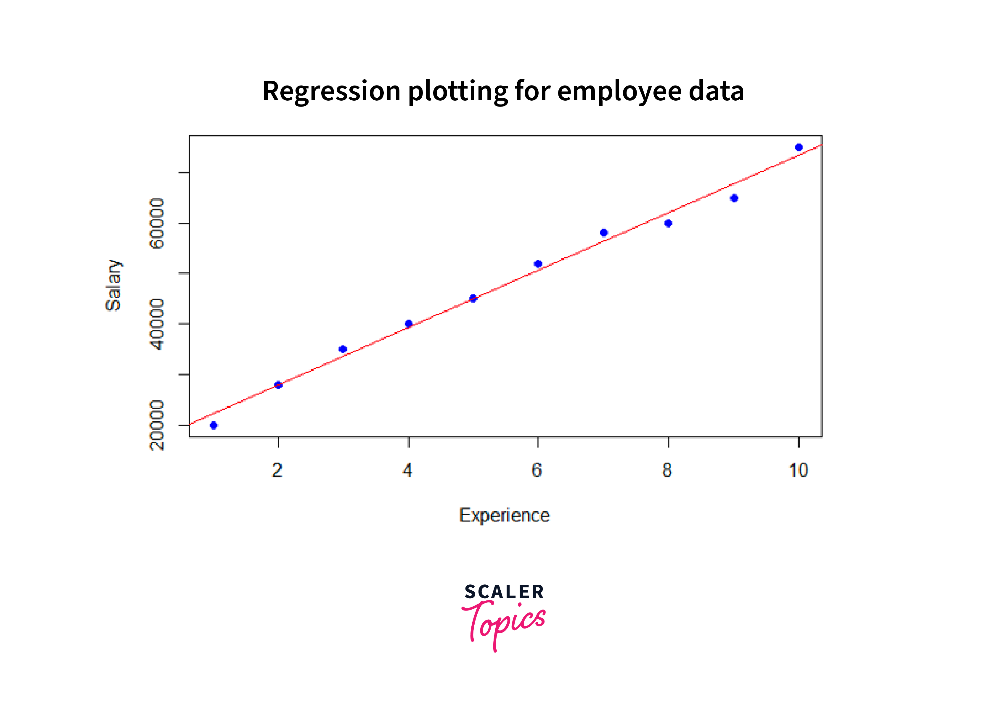
Next, we'll visualize the relationship between the variables using a regression plot in R.

Output:

Here we used the plot() function to create the scatter plot, specifying the "experience" as the x-axis and "salary" as the y-axis. The pch parameter sets the shape of the points to 16, and the col parameter sets the color of the points to blue. Finally, we used the abline() function to add the regression line to the plot, which takes the linear regression model, model, as an argument created using the lm() function and sets the line's color as red.