Matrix Chain Multiplication

Introduction to Matrix Chain Multiplication

In linear algebra, matrix chain multiplication is an operation that produces a matrix from two matrices. But, multiplying two matrices is not as simple as multiplying two integers, certain rules need to be followed during multiplying two matrices.

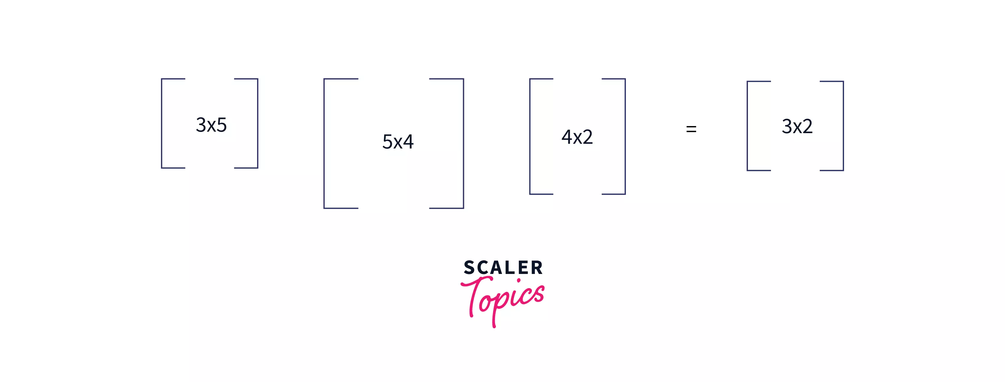
Let's say we have two matrices, $X$ of dimensions $x_1\times x_2$ and $Y$ of dimensions $y_1\times y_2$. $X$ and $Y$ can be multiplied if and only if $x_2=y_1$. And if the condition satisfies the resultant matrix (say $P$) will be of dimension $x_1\times y_2$ and it requires $x_1\times x_2 \times y_2$ multiplication steps to compute $P$.

If we have been given a chain of matrices of some arbitrary length '$n$', the number of multiplication steps required to multiply all the matrices highly depends on the order in which we multiply them.

So, in the matrix chain multiplication problem, we have been given an array representing the dimension of matrices $[M_1, M_2, ... , M_n]$ and we are interested to deduce the minimum number of multiplication steps required to multiply them.

Example of Matrix Chain Multiplication

We have studied in our school days that matrix chain multiplication follow associative rule $i.e.$ KaTeX parse error: $ within math mode and the number of steps required in multiplying matrix $M_1$ of dimension $x\times y$ and $M_2$ of dimension $y\times z$ are $x\times y\times z$, and the resultant matrix $M_{12}$ is of dimension $x\times z$

Let's assume we have three matrices $M_1, M_2, M_3$ of dimensions $5\times 10$, $10\times 8$, and $8\times 5$ respectively and for some reason we are interested in multiplying all of them. There are two possible orders of multiplication -

• $M_1\times(M_2\times M_3)$
  • Steps required in $M_2\times M_3$ will be $10\times 8\times 5$ $=$ $400$.
  • Dimensions of $M_{23}$ will be $10\times 5$.
  • Steps required in $M_1\times M_{23}$ will be $5\times 10 \times 5$ $=$ $250$.
  • Total Steps $=$ $400+250$ $=$ $650$
• $(M_1\times M_2)\times M_3$
  • Steps required in $M_1\times M_2$ will be $5\times 10\times 8$ $=$ $400$.
  • Dimensions of $M_{12}$ will be $5\times 8$.
  • Steps required in $M_{12}\times M_{3}$ will be $5\times 8 \times 5$ $=$ $200$.
  • Total Steps $=$ $400+200$ $=$ $600$

Here, if we follow the second way, we would require $50$ fewer operations to obtain the same result.

Hence, it is necessary to know the optimal way in order to speed up the multiplication process by placing the brackets at every possible place and then checking which positioning minimizes the effort.

Naive Recursive Approach

The idea is very simple, placing parentheses at every possible place. For example, for a matrix chain $M_1 M_2 M_3 M_4$ we can have place parentheses like -

• $(M_1)(M_2M_3M_4)$
• $(M_1M_2)(M_3M_4)$
• $(M_1M_2M_3)(M_4)$

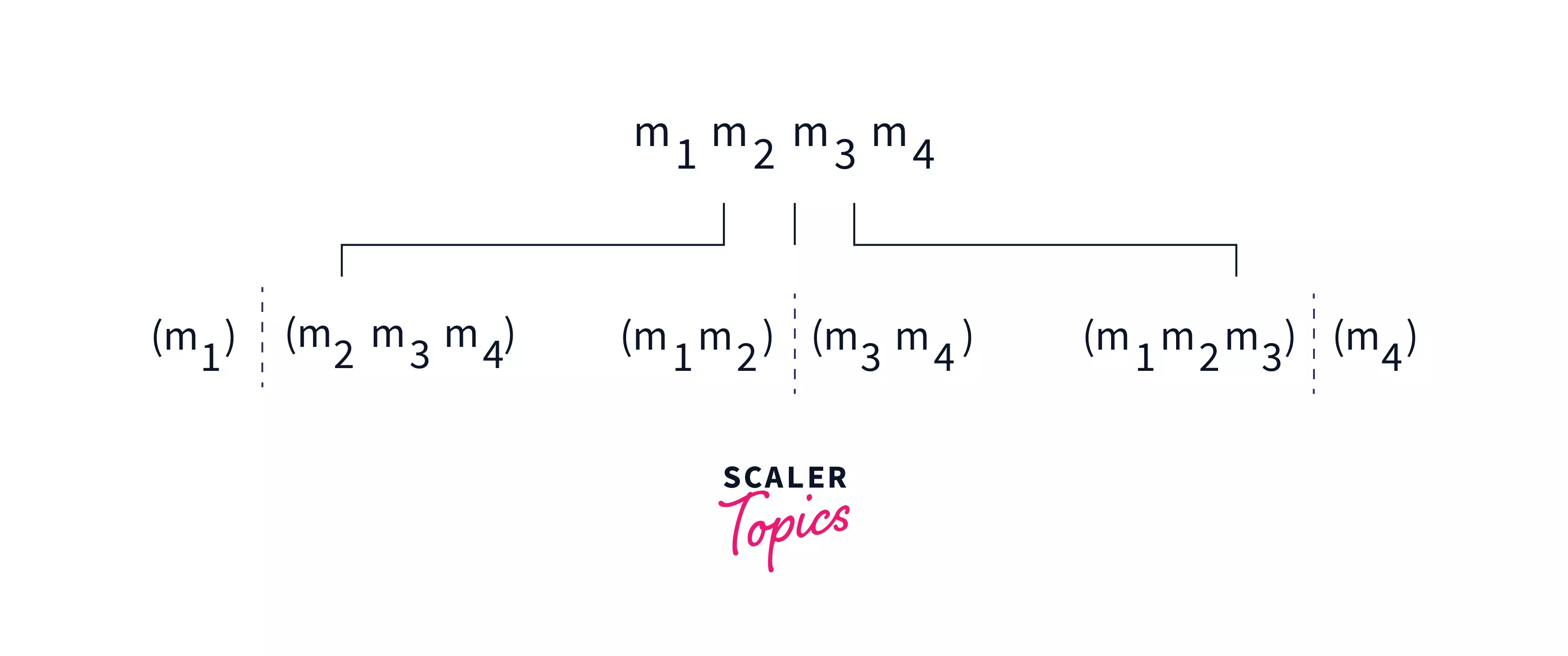
So for a matrix chain multiplication of length $n$, $M_1M_2...M_n$ we can place parentheses in $n-1$ ways, notice that placing parentheses will not solve the problem rather it will split the problem into smaller sub-problems which are later used to find the answer for the main problem.

Like in $(M_1)(M_2M_3M_4)$ the problem is divided into $M_1$ and $(M_2M_3M_4)$ which can be solved again by placing parentheses and splitting the problem into smaller sub-problems until size becomes less than or equal to 2.

So we can deduce the minimum number of steps required to multiply a matrix chain of length $n$ $=$ minimum number of all $n-1$ sub-problems.

To implement it we can use a recursive function in which we will place parentheses at every possible place, then in each step divide the main problem into two sub-problems $i.e.$ left part and right part.

Later, the result obtained from the left and right parts can be used to find the answer of the main problem. Let's have a look at Pseudocode for better understanding.

Pseudocode of Recursive Approach

Explanation - To implement the matrix chain multiplication algorithm we can have a recursive function MatrixChainMultiplication which accepts three arguments $i.e.$ an array (say mat) of integers representing dimensions of the matrices, low representing the starting index of the current sub-problem (initially low will be 0), and high representing the last index of the current sub-problem.

• The base case of this recursive function occurs when we will reach low$=$high because it means we are left with a sub-problem of size 1 $i.e.$ a single matrix $M_i$ so we will return 0.
• Then, we will iterate from low to high and place parentheses for each i such that low$\leq i<$high.
• During each iteration we will also calculate the cost incurred if we place at that particular position $i.e.$ Cost of left sub-problem + cost of right sub-problem + mat[low-1]$\times$mat[k]$\times$mat[high]
• At last we will return the minimum of the costs found during the iteration.

C/C++ Implementation of Recursive Approach

Java Implementation of Recursive Approach

Output -

Complexity Analysis

• Time Complexity - Let $T(n)$ be the total number of ways to place parentheses in the matrix chain, where $T(n)$ is defined as -

  $T(n)= \begin{cases} \Sigma^{n-1}_{i=1} \hspace{0.2cm} T(i) + T(n-i), &\text{if } n\geq2 \\ 1, & \text{if } n=1 \end{cases}$

  On solving the above given recurrence relation, we get - $T(n)=O(2^n)$ which grows at an exponential rate.

• Space Complexity - Though we have not used any auxiliary space but as you can see in the above image, the maximum depth of the recursive tree can reach up to $O(n)$ where $n$ is the length of the matrix chain. Hence the overall space complexity is $O(n)$

Need of Dynamic Programming

If we closely observe the recursive tree that is formed during finding the multiplication order, we will find that the result of the same sub-problem had been calculated many times also many overlapping sub-problems can be seen in the recursive tree.

For example, in a matrix chain of length 4, the recursive tree formed looks like -

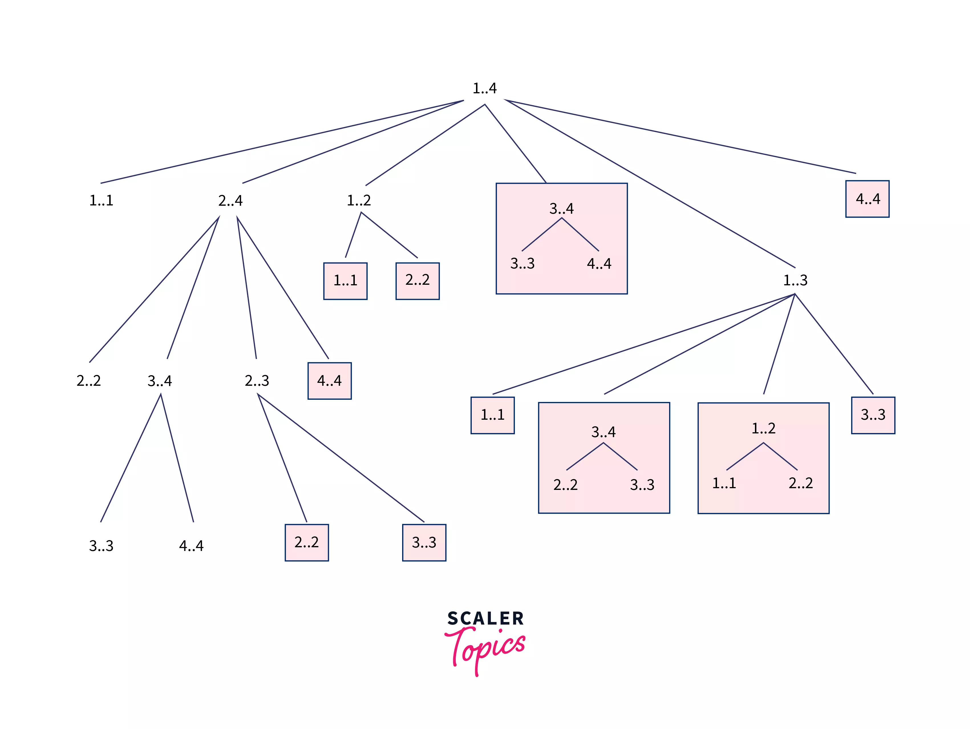
We can see that answers for the sub-problem $1..2$, and $2..3$ have been calculated two times. So if we store them somewhere it will highly beneficial to speed up the process.

All these things suggest using Dynamic programming to find an efficient solution.

DP With Memoization

Algorithm for DP Using Memoization

The algorithm is almost the same as the naive recursive solution with the only change that here we will use a $dp$ array of dimension $n\times n$.

Steps -

• Declare a global $dp$ array of dimension $n\times n$ and initialize all the cells with value $-1$.

• $dp[i][j]$ holds the answer for the sub-problem $i..j$ and whenever we will need to calculate $i..j$ we would simply return the stored answer instead of calculating it again.

• Initialize variables low with $1$, and high with $n-1$ and call the function to find the answer to this problem.

• If $low=high$ then return 0 because we don't need any step to solve sub-problem with a single matrix.

• If $dp[low][high] \neq -1$ it means the answer for this problem has already been calculated. So we will simply return $dp[low][high]$ instead of solving it again.

• In the other case, for each $i=low$ to $i=high-1,$ we will find the minimum number of steps in solving the left sub-problem, right sub-problem, and steps required in multiplying the result obtained from both sides. Store the result obtained in dp[low][high] and return it.

• At last answer for $low=0$ and $high=n-1$ $i.e.$ $dp[0][n-1]$ will be returned.

Pseudocode

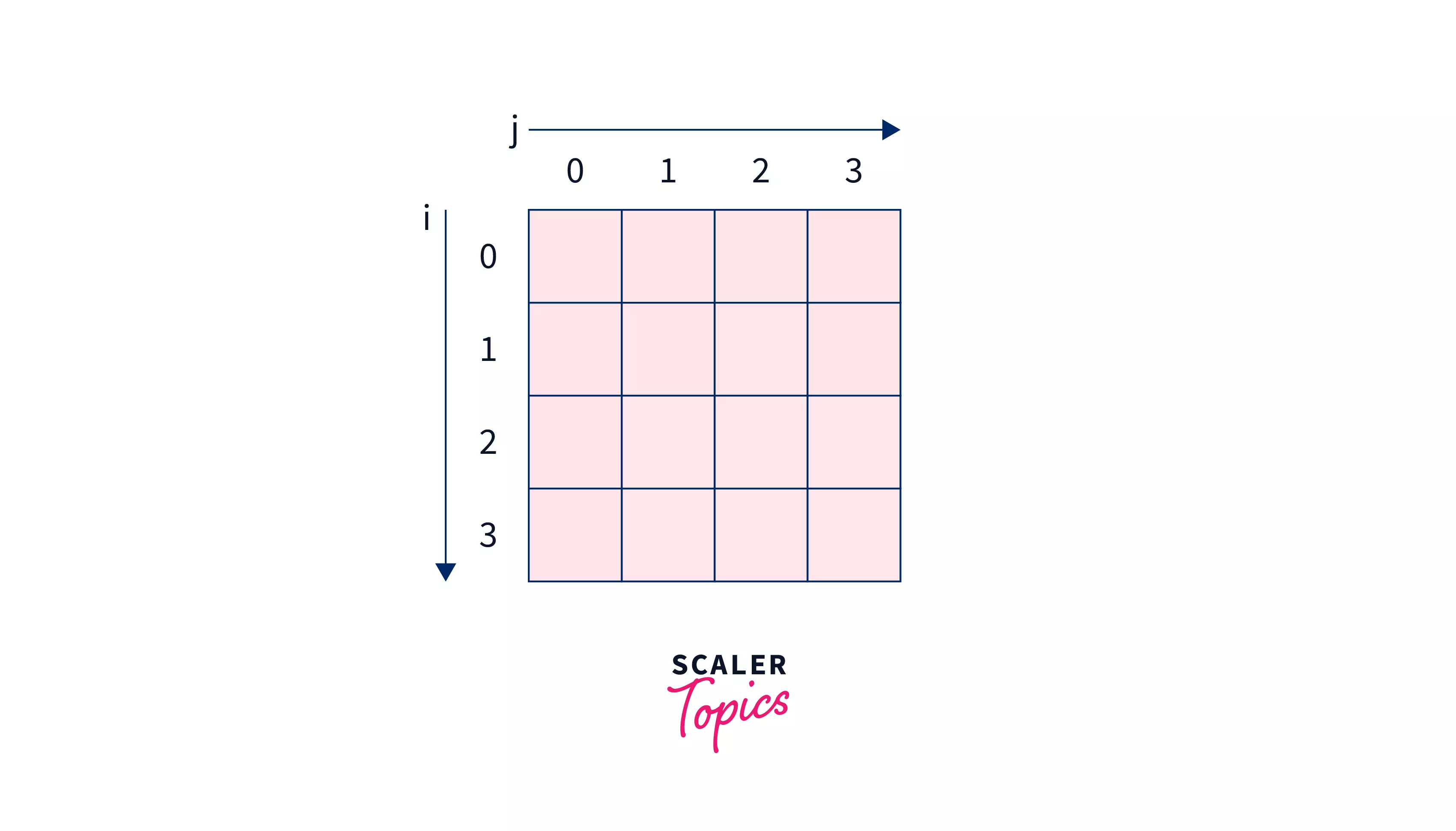
Explanation - We will use almost the same approach as Recursive Implementation with the only change that, we will maintain a 2-D array (say dp) of dimensions $n\times n$ all of whose entries initialized with -1 where dp[i][j] stores result for the sub-problem i..j.

So for calculating the answer for the sub-problem i..j firstly we will check if we already have calculated the answer for it in past, by checking that if dp[i][j]!=-1. So if we already have calculated the answer for it we need not solve it again instead, we can simply return dp[i][j]

C/C++ Implementation

Output -

Complexity Analysis

• Time Complexity - In the function we are iterating from $1$ to $n-1$ which costs $O(n)$ and in each iteration, it takes $O(n^2)$ time to calculate the answer of left and right sub-problems. Hence, the overall time complexity is $O(n^3)$

• Space Complexity - We are using $dp$ array of dimension $n\times n$. So the space complexity is $O(n^2)$

Bottom-up DP Solution

Algorithm

To solve this problem in a Bottom-up manner we will be following the "Gap strategy". Gap strategy means firstly we will solve all the sub-problems with gap=0, then with gap=1, and at last problem with gap=n-2.

For solving a problem with gap $i$ such that $i\geq2$, all the problems of size $i-1$ will be taken into account. Please refer to the following algorithm and example for a better understanding.

• For sub-problem with gap 0 (single matrix), no multiplication is required so the answer will be 0.
• For sub-problem with gap 1 (two matrices $i.e.$ A and B) the only option is to simply find steps required in multiplying A and B.
• For sub-problems with gap$\geq2$ we need to find the minimum by placing the brackets at all the possible places.

For example -

• Answer for the sub-problem $\{i,j\}$, when $i=j$ is 0.
• Answer for the sub-problem $\{i,j\}$, when $j-i=1$ is $mat[i]\times$ $mat[j]\times mat[j+1]$.
• Answer for the sub-problem $\{i,j\}$, when $(j-i)\geq2$, is obtained by placing bracket at all possible places, and then calculating the sum of left sub-problem, right sub-problem and cost of multiplying matrices obtained from left and right side.

Pseudocode

Let's dry run this algorithm on $mat=\{2, 4, 6, 8, 6\}$.

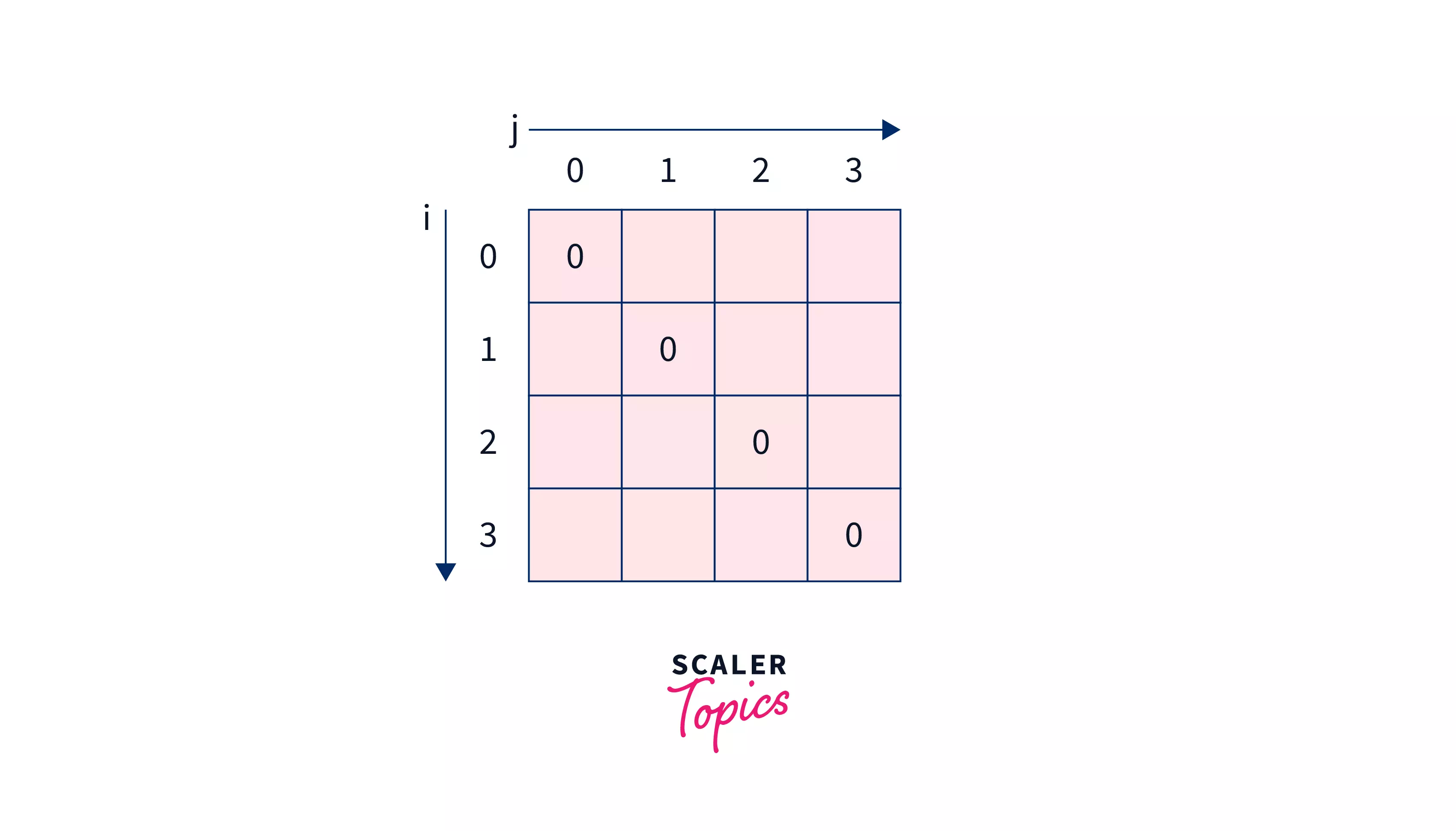
Here the length of the chain is 5, so we will create $dp$ array of dimension $4\times 4$ as shown below -

Then solving sub-problems of size $0$ $i.e.$ $\{0,0\},$ $\{1,1\},$ $\{2,2\},$ and $\{3,3\}$. As per the algorithm all of them will result in 0. After which $dp$ array will look like -

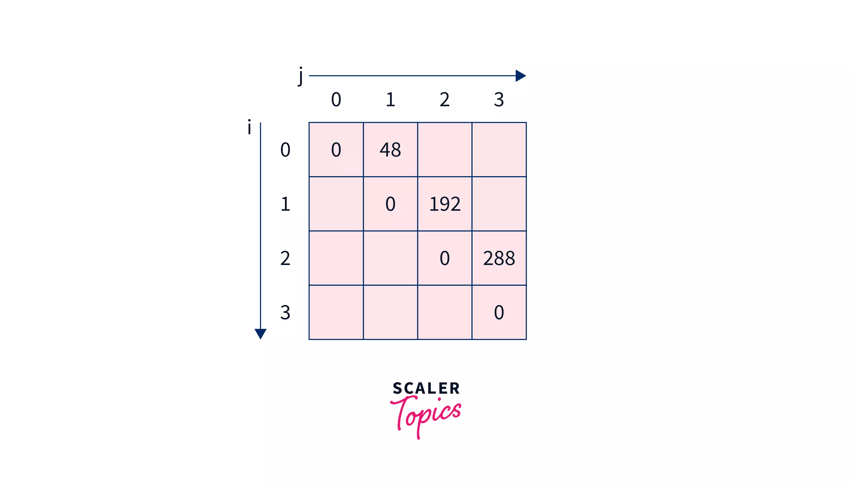
Solving all sub-problems of gap $1$ $i.e.$ $\{0,1\},$ $\{1,2\},$ and $\{2,3\},$.

• $\{0,1\}$ will result in $2\times 4\times 6$ $=48$
• $\{1,2\}$ will result in $4\times 6\times 8$ $=192$
• $\{2,3\}$ will result in $6\times 8\times 6$ $=288$

After which $dp$ array will look like -

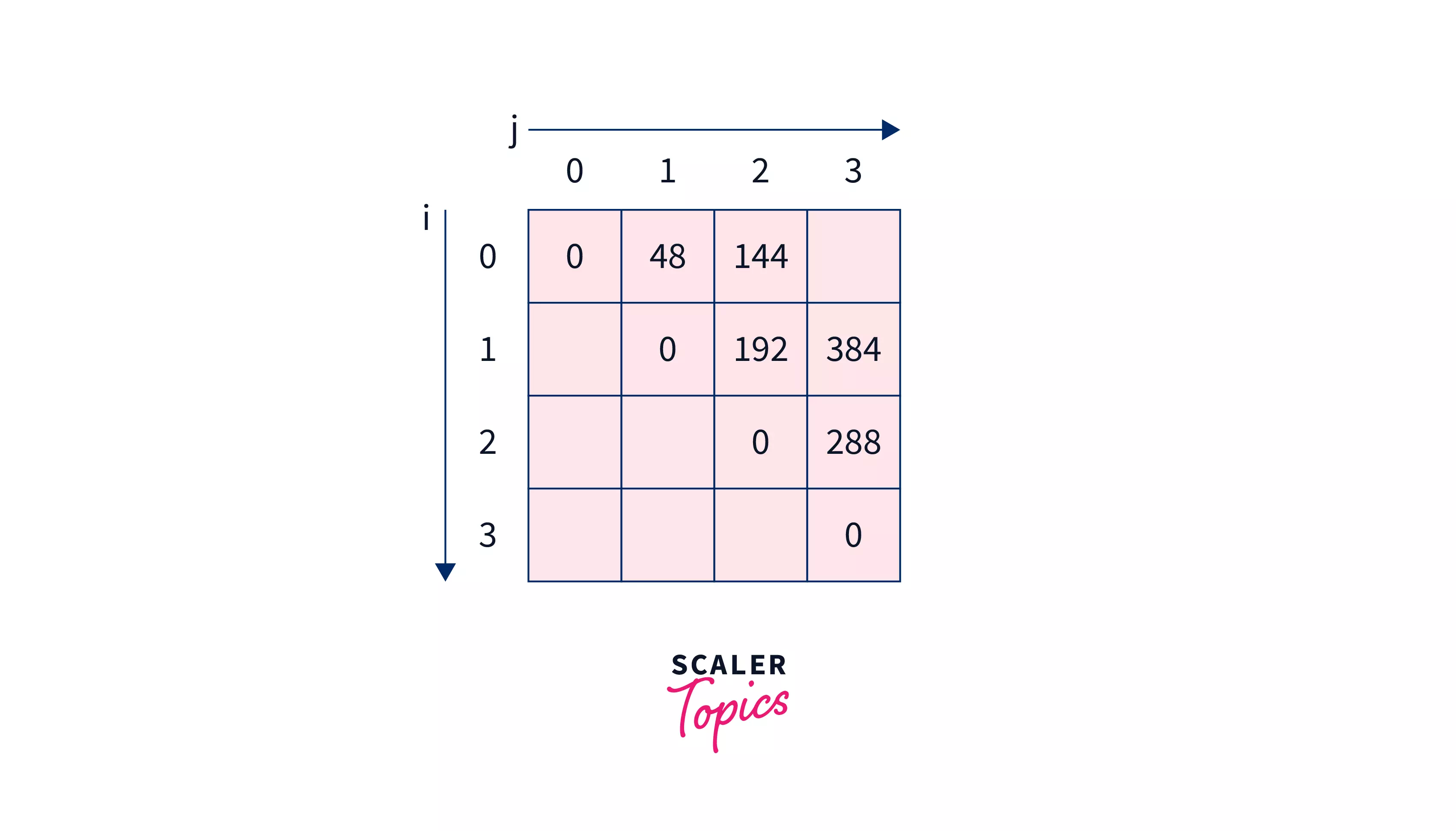
Now solving sub-problems with gap $2$ $i.e.$ $\{0,2\}$ and $\{1,3\}$.

• $\{0,2\}$ will result in minimum of -

  • $dp[0][0]+dp[1][2]+(2\times 4\times 8)= 0 + 192 + 64=256$
  • $dp[0][1]+dp[2][2]+(2\times 6\times 8)=48+0+96=144$

  Hence we will make $dp[0][2]$ as $144$.

• $\{1,3\}$ will result in minimum of -

  • $dp[1][1]+dp[2][3]+(4\times 6\times 6)= 0 + 288 + 144=432$
  • $dp[1][2]+dp[2][2]+(4\times 8\times 6)= 192 + 0 + 192=384$

  Hence we will make $dp[1][3]$ as $384$

Now solving the last problem (main problem) with gap 3 $i.e.$ $\{0,3\}$. It will be minimum of -

• $dp[0][0]+dp[1][3]+(2\times 4\times 6)= 0 + 384 + 48=432$
• $dp[0][1]+dp[2][3]+(2\times 6\times 6)= 48 + 288 + 72=408$
• $dp[0][2]+dp[3][3]+(2\times 8\times 6)= 144 + 0 + 96=240$

So 240 is the minimum among them, hence we will make $dp[0][3]$ as 240 making $dp$ array look like -

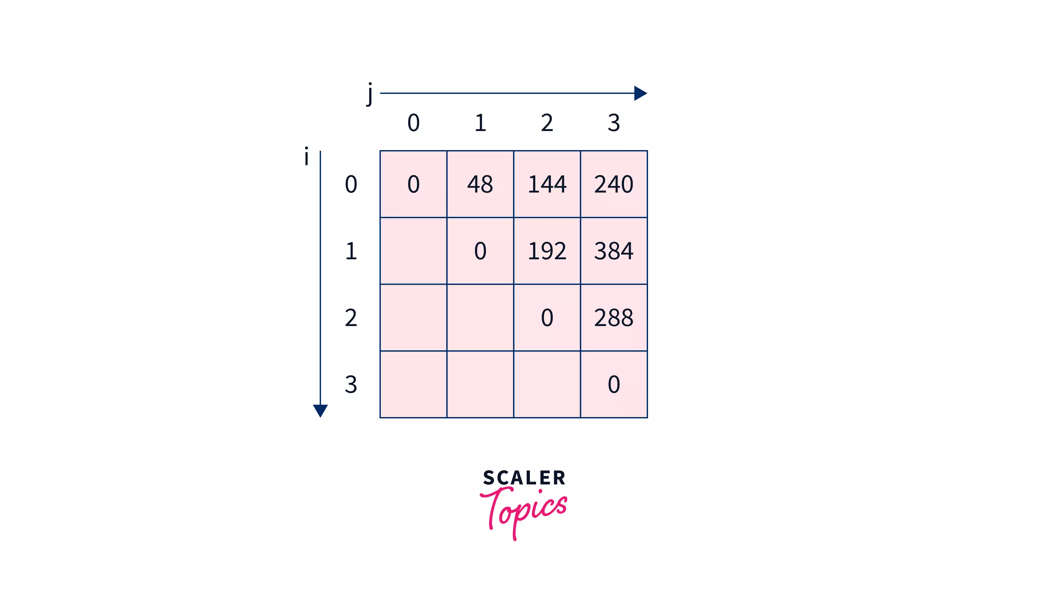
At last we will return $dp[0][5-2]=dp[0][3]$ $i.e.$ $240$.

C/C++ Implementation

We will use a 2-D array (say $dp$) of dimensions $(n-1)\times(n-1)$ because the last problem is of size/gap $n-2$. Then we will iterate for each sub-problem with gap/size $0$ till the last problem with gap/size $n-2$ and compute the answer for the sub-problem based on the rules discussed in the algorithm section. At last, the answer of the final problem will be stored in $dp[0][n-2]$ so we will simply return it.

Output -

Complexity Analysis

• Time Complexity - We are using three nested for loops, each of which is iterating roughly $O(n)$ times. Hence, the overall time complexity is $O(n^3)$.
• Space Complexity - We are using an auxiliary $dp$ array of dimensions, $(n-1)\times(n-1)$ hence space complexity is $O(n^2)$

Join our expert-led Free Dynamic Programming Course to master advanced problem-solving techniques and enhance your programming prowess.