Cost Risk Analysis- Monte Carlo Simulation in Excel : What should you use?

What Are We Building?

We are building a model, Cost Risk Analysis- Monte Carlo Simulation, in Excel.

• The Monte Carlo approach aims to improve data analysis using random data sets and probability computations.
• Excel and a dice game can create a Monte Carlo simulation.
• The results can be generated using a data table; 5,000 results are required to set up the Monte Carlo simulation.

Pre-requisites

Monte Carlo Simulation

In the 1940s, John von Neumann and Stanislaw Ulam developed the Monte Carlo method, which uses random and probabilistic approaches to tackle complicated problems. The Monaco administrative district, popularly recognized as a gambling hotspot for European aristocracy, is called Monte Carlo.

The Monte Carlo simulation method introduces a statistical perspective on risk in a probability decision by computing the probability for integrals and solving partial differential equations. Although numerous complex statistical programs are available to produce Monte Carlo simulations, it is simpler to model the uniform and normal laws using Microsoft Excel and avoid the mathematical fundamentals.

Project Risk Analysis

Risk analysis utilizes methods and procedures to ascertain the possibility and consequences of previously identified project hazards. Therefore, risk analysis aids project managers in understanding the unpredictability of potential hazards and how, if they materialize, they will affect the project's schedule, quality, and costs.

You should use project management software for risk analysis because projects will always exist, regardless of your business. For instance, ProjectManager provides risk management capabilities that enable real-time risk tracking. Keep track of specific risk incidents, and use project dashboards to monitor your project's overall risk.

Cost Risk Analysis

An early estimate of probable cost overruns and the cost components with probability distributions that have the greatest influence on these outcomes can be given to program management by a CRA.

Schedule Risk Analysis

Schedule Risk Analysis (SRA) assesses a schedule's viability and chances of accomplishing the project's stated objectives. Due to its quantitative nature and mathematical foundation, it allows the project to track potential schedule delays during the course of the project.

Sensitivity Analysis

Sensitivity analysis is a type of financial model that assesses the impact of changes in input variables on target variables. It is a technique for forecasting a decision's outcome given a set of relevant factors.

How Are We Going to Build This?

• Start the statistics table
• Create the data table and give it a name.
• Summarise the data table's findings.
• Finish the statistics table.
• A Summary of the Monte Carlo Prediction
• Create the Section for Projected Net Profit.
• Put together the Key Percentiles Section.
• Bringing the Monte Carlo Analysis to a Close

Final Output

Requirements

Monte Carlo simulation is made possible by this add-in, MCSim.xla, from an Excel sheet. The add-in recalculates the sheet as many times as you choose when you choose a cell that contains or depends on a random number (using either Excel's RAND or our RANDOM function). It writes the results on a new sheet with a histogram and summary statistics. Numerous other settings are available, and you can use Monte Carlo in more than one cell.

Excel's data analysis tool, Random Number Generation, generates random numbers in a table that follows one of several distributions in addition to the RAND and RANDBETWEEN functions. With this tool, you can specify the following values:

Samples are equal to the number of variables. This is the number of columns in Excel's output table.

Size of each sample = Number of Random Numbers. This is the number of rows in the Excel output table.

Choose the desired distribution from the list of distributions below:

• Describe the (lower bound) and (upper bound) uniformly
• Please provide the mean and standard deviation for normal.
• Like the binomial distribution with n = 1, Bernoulli should state the probability of success (p).
• Binomial, specify n trials and p (probability of success)
• (Mean) Poisson
• Patterned:
  Specify a step, a repetition rate for the values, a repetition rate for the sequence, a lower and upper bound, and more.
• Specify a value and the corresponding probability range. The range must have two columns: the right column must contain probabilities related to each value in the row, and the left column must contain values. The probabilities must add up to 1. Thus, they must.

An optional variable called a "random seed" produces the initial random number. Again, you can use this value to guarantee that the same random numbers are generated. A fresh random number will be produced each time this field is left empty.

Cost Risk Analysis in Excel

Data Collection and Preparation

A beginning amount, forecasts for returns and expenses over several years, and a closing balance at some point in the future are all components of a conventional investment portfolio model. A simple spreadsheet model might look like this:

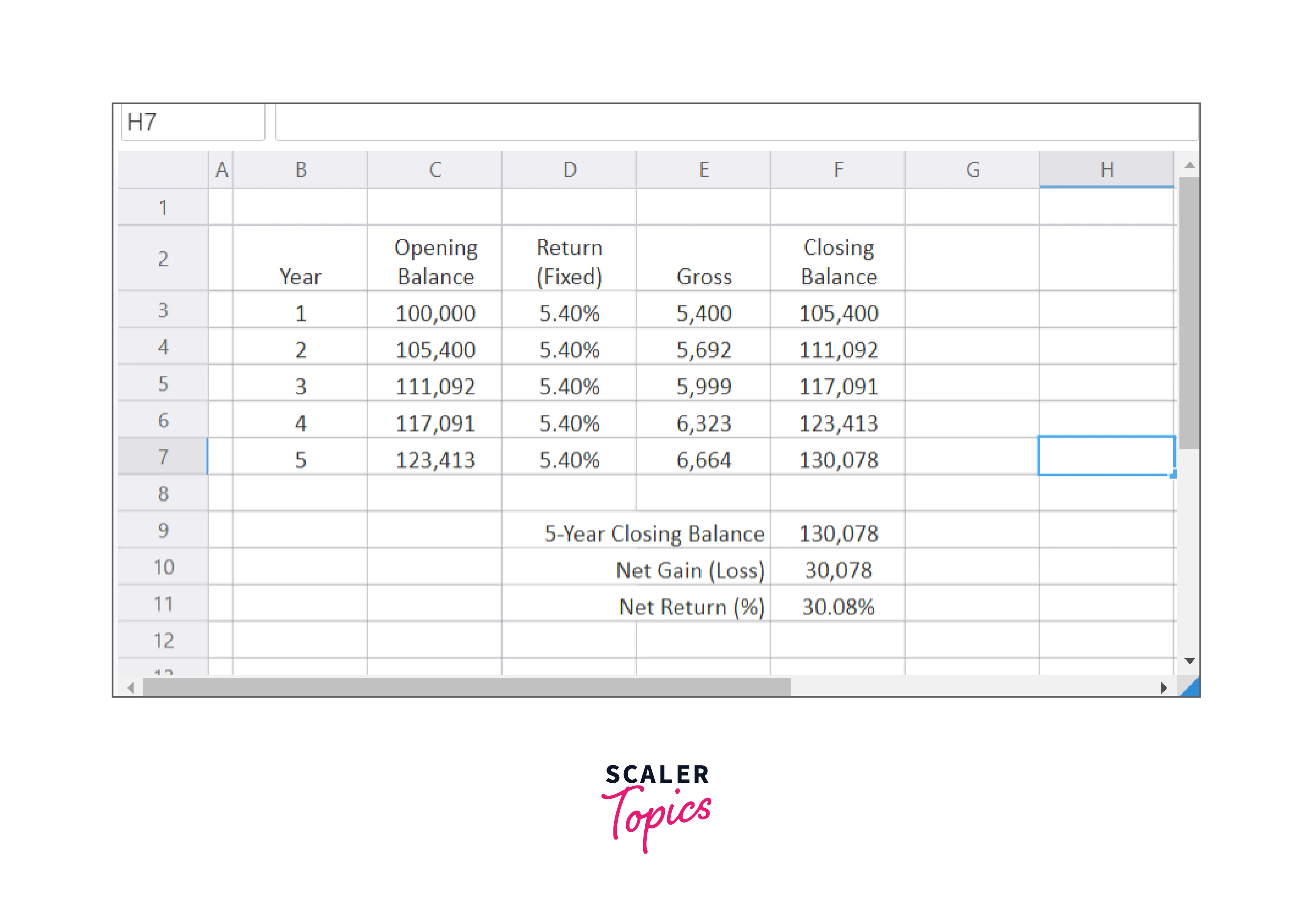
The model in Figure A is based on a yearly return of 5.4% over a set time. This yields a return over a 5-year period of 30.08%.

Although a return of 5.4% will be expected, we know that actual returns can vary substantially. To more closely resemble reality, these fixed returns are initially replaced with randomly distributed values before constructing the Monte Carlo model.

Define the Project Cost Variables

Instead of a fixed return of 5.4% in the Monte Carlo model, we expect a normally distributed return, with a mean (average) of 5.4% and a standard deviation of 7.3%. Column D of the spreadsheet has return cells, and we use the random function NormalValue for each.

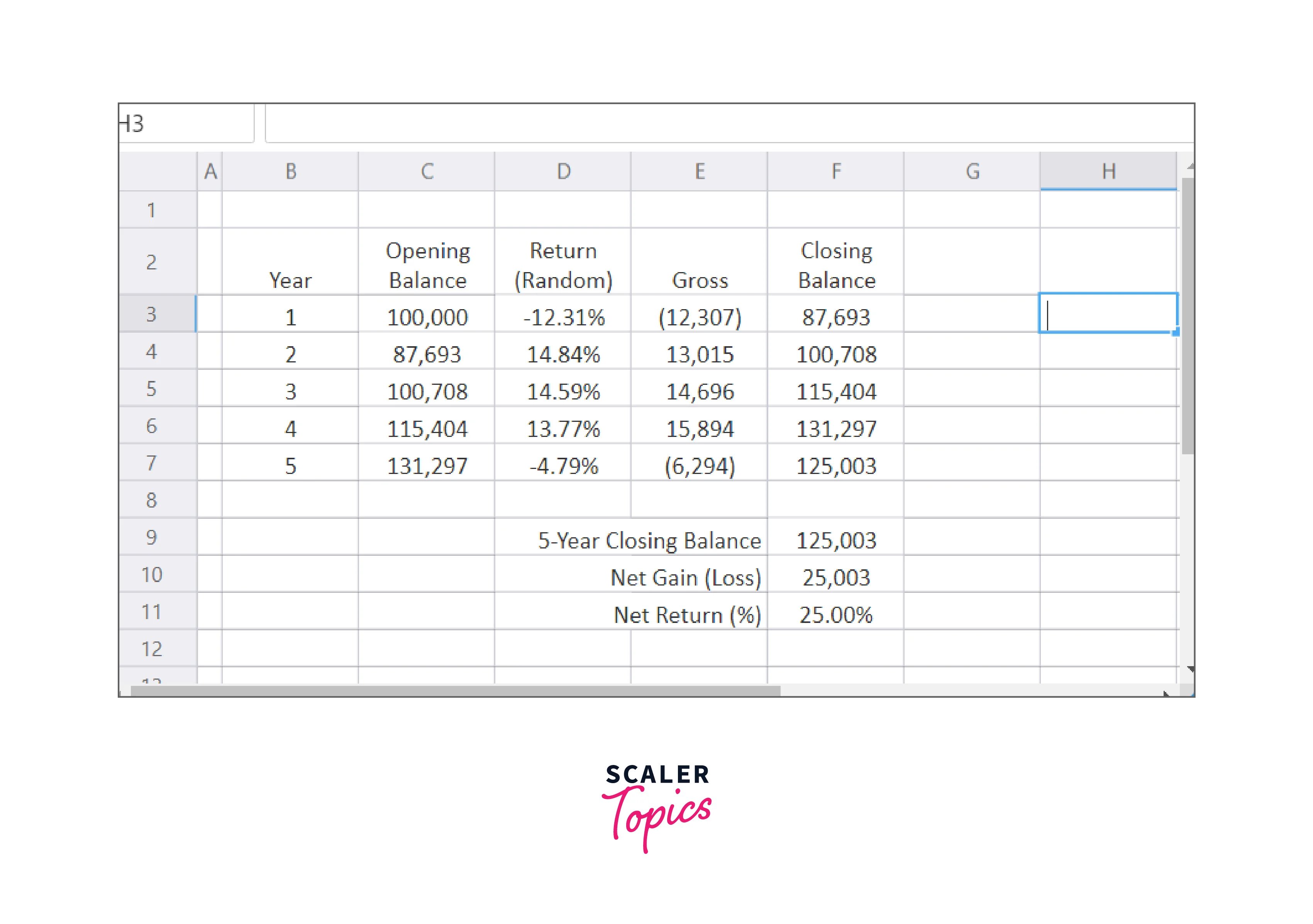
Using the function visible in the function bar, the return in each period of Figure B has been modified from a fixed 5.4% to a randomly dispersed return. Each period's returns are determined at random. You can recalibrate the model at this stage to check how each return has changed. The total return (F11) can also deviate greatly from the starting point (30.08%).

Randomly distributed returns better represent the real world, yet taking just one random return is useless. The secret to using Monte Carlo simulation is to run the model several times with random values, then examine the outcomes.

Create a Monte Carlo Simulation Model

A Monte Carlo simulation runs the same model numerous times with the goal of extracting information that can be used. Click the "Play" button next to the spreadsheet to launch a Monte Carlo simulation. Use the Monte Carlo toolbar's "Run Simulation" button in Excel.

Run the Monte Carlo Simulation

Various functions are included in the add-in to analyze the outcomes of a Monte Carlo simulation. We'll first examine the simulation's average outcomes using the SimulationMean function.

A #N/A error will appear when you insert these functions for the first time in a spreadsheet. This is due to the simulation not having yet gathered data for the cell. This error will disappear when you execute a simulation.

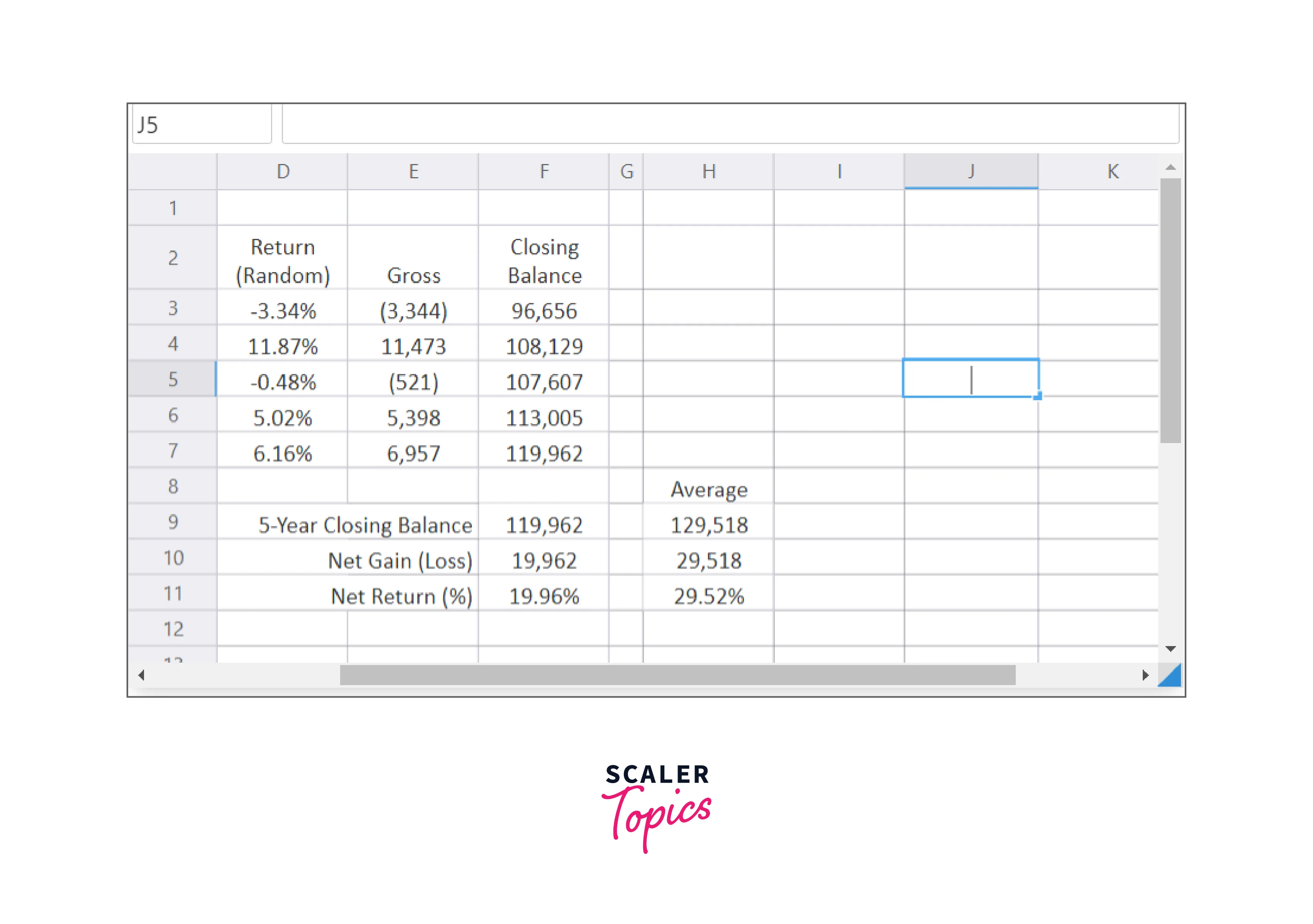
Using the function shown in the function bar, we put the average simulation results in column H of Figure C. The average value of cell F11 over all trials, or iterations, of the Monte Carlo simulation is determined in this example's cell H11.

When you do a Monte Carlo simulation, the spreadsheet is updated, and new random values are added to column D at each iteration. As a result, cell F11 now has a different value. The Add-in stores and remembers the value of cell F11 at each iteration of the Monte Carlo simulation, which occurs hundreds or thousands of times. This collection of recorded values can be used to calculate the average value after the simulation.

You can see that the average value displayed in cell H11 is quite similar to the fixed initial value of 30.08% (see cell F11 in Figure A). This is in line with expectations, given that the fixed number in the original model, 5.4%, was fixed in the random data we're utilizing for returns.

Analyze the Simulation Results

As previously mentioned, the Monte Carlo simulation's average return is very similar to the fixed model's initial return. The simulation wouldn't be very useful if it were the only thing we could learn from. However, we can glean far more pertinent information from the Monte Carlo simulation by examining ranges and percentiles.

First, using the SimulationMin and SimulationMax functions, we can examine the minimum and maximum values determined throughout the simulation:

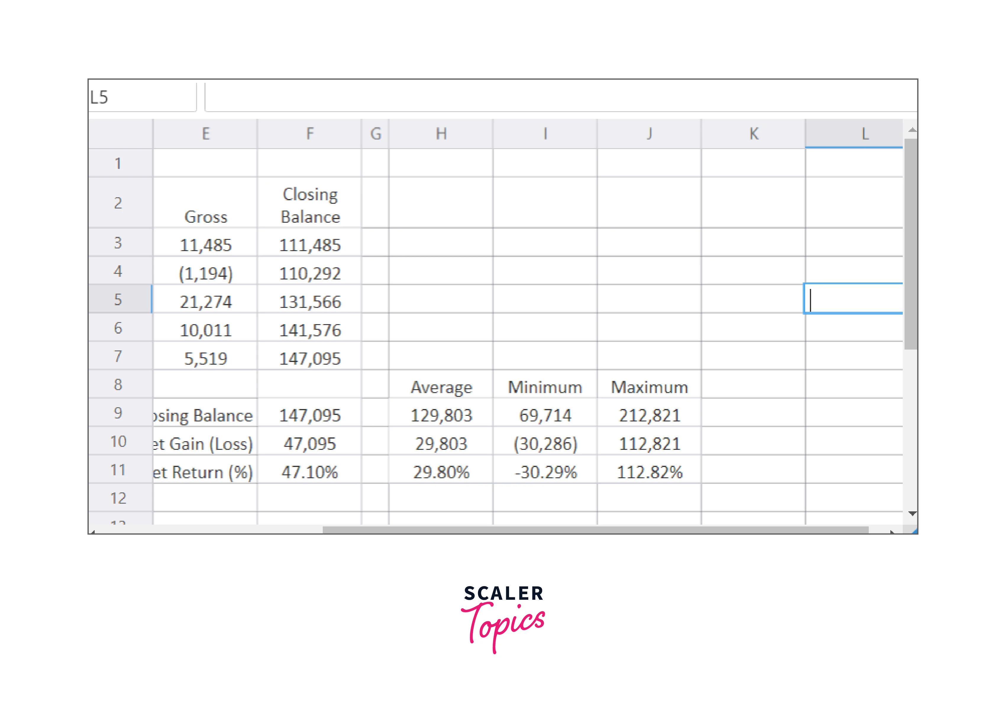
The simulation's minimum value for cell F11 is represented in cell I11 of Figure D. This shows the risk in the portfolio model and is significantly greater than the average. This indicates that this portfolio may see a net loss of 33% over the course of five years.

The outliers, or tails, of the portfolio model's potential outcomes tend to be overstated when considering only the absolute minimum and maximum values. Using the SimulationPercentile function, we can also examine percentile probabilities:

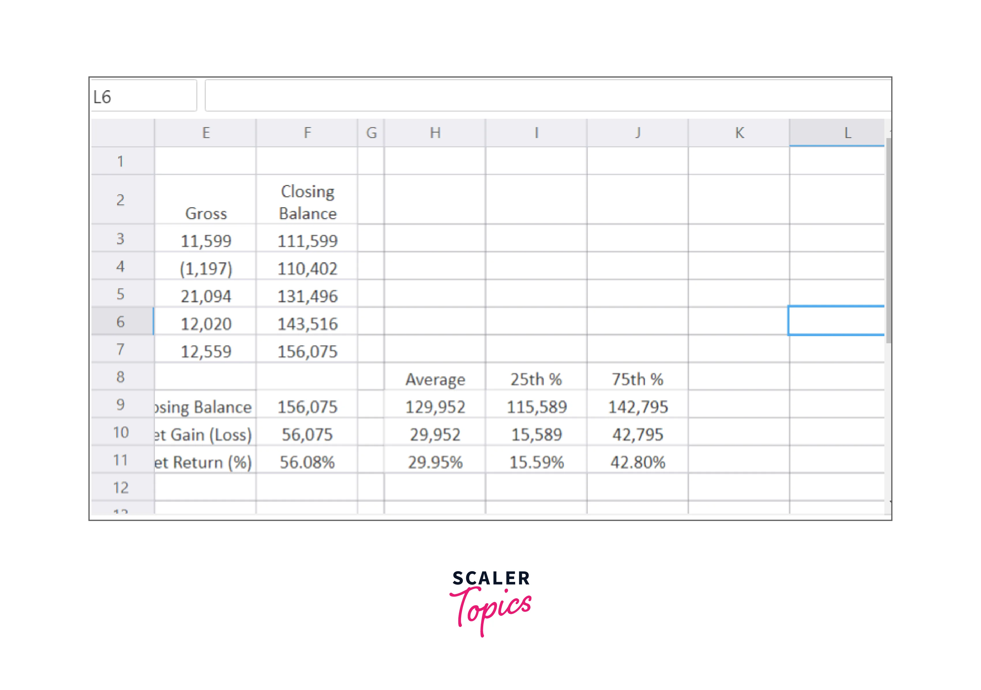
The SimulationPercentile function is present in cell I11 of Figure E, as indicated by the function bar. Imagine that we rank all of the Monte Carlo simulation results observed in cell F11 from lowest to highest to comprehend what the percentiles signify. As can be seen from the example above, the first value is the minimum; no other values in the results are lower than the minimum value. The maximum would be the last value; 100% of the results' values are equal to or less than the last value. The 100th Percentile is, therefore, the highest value.

Therefore, a value equal to or more than 25% of the simulation's results is represented by the 25th Percentile. In other words, there is a 25% probability that any simulation value will be lower than or equal to this amount and a 75% chance that it will be higher than or equal to this amount.

Cell I11 in Figure E displays the 25th percentile outcome for cell F11. This indicates that, during the simulation, the value of F11 is greater than or equal to 16.61% 75% of the time. The probability that our model will produce a total return of at least 16.61% is 75%.

We may calculate the portfolio's expected to return with various probabilities by varying the percentile values. This type of study can help determine the actual risk levels connected to a portfolio of investments.

Perform Sensitivity Analysis

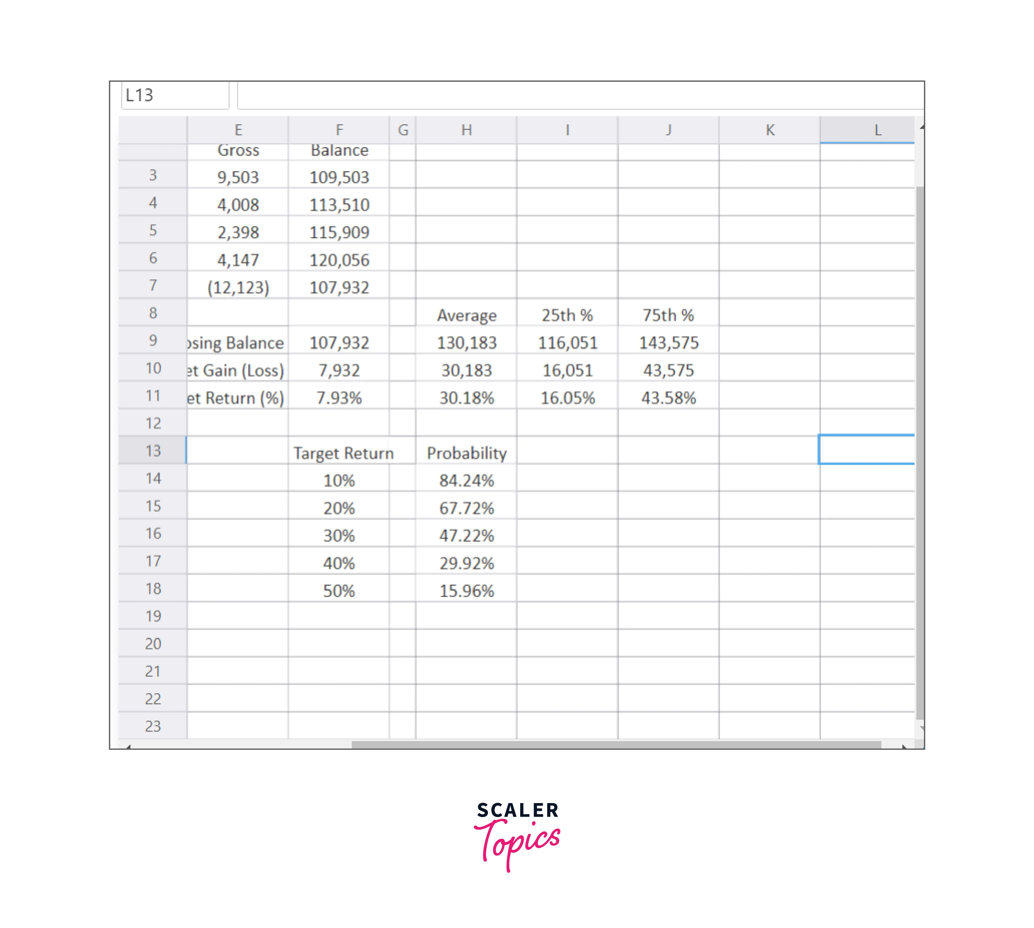
With the SimulationInterval function, we can use the analysis to find the probability of achieving a specific goal return rather than determining the expected return at various percentiles:

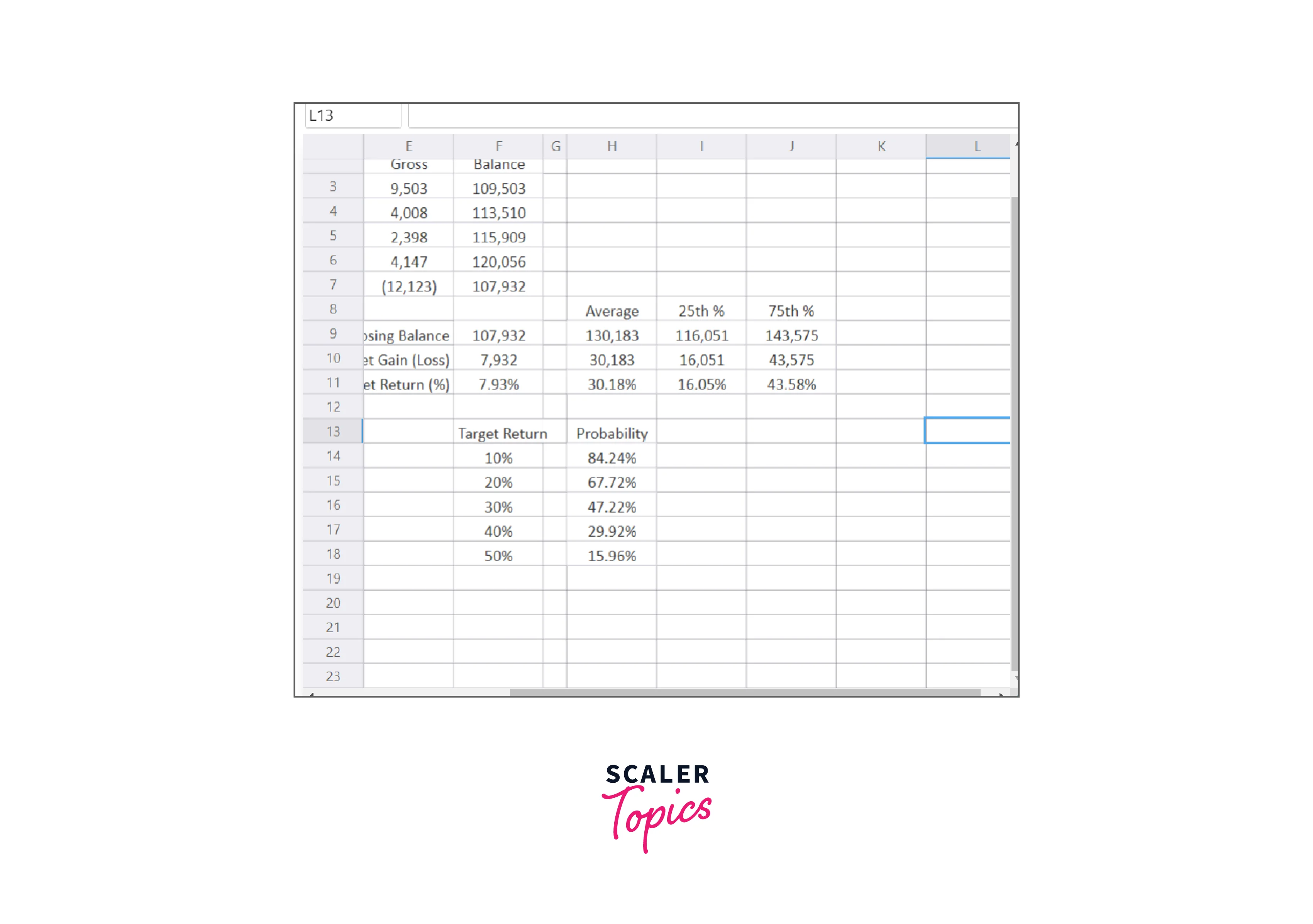
What is the probability that the model will return at least 50% overall simulation trials, according to this analysis?
This probability is around 16% in Figure F, meaning there is a 16% chance the model will produce a return of 50% or more.

Confidence levels can be determined using this type of analysis. For instance, we can contrast the probability of achieving specific minimal returns while assessing alternative investments. Alternatively, we can determine the possibility that an investment will yield 0% to comprehend the risk of loss involved.

Remember that the exact percentage will vary depending on the simulation you perform, although it will always be close to 16% in this model.

Develop Risk Mitigation Strategies

We employ the Monte Carlo approach when an issue is too complex and challenging to solve through direct calculation. The simulation can be used to help find solutions in unclear situations. The normal distribution can be simulated with a lot of iterations. It can also be utilized to appreciate the uncertainty in forecasting models and how risk functions.

As previously mentioned, simulation is frequently used in various fields, including finance, research, engineering, and supply chain management—particularly when there are excessive random variables at play. For instance, analysts may use Monte Carlo simulations to assess derivatives, such as options, or to assess risks, such as the possibility that a company may fail to make its debt payments.

Testing

The best way to understand Monte Carlo simulations is to imagine a person rolling dice. The probabilities of rolling a six in any combination, like four and two, three and three, or one and five, will be completely unknown to a new player at craps. The probability of rolling a "hard six," often known as two threes, is what? We can determine the likelihood that a roll of six will be a hard six by rolling the dice a large number of times, ideally several million times. We want to execute these tests as rapidly and effectively as possible, and a Monte Carlo simulation does that.

Dice rolls do not determine future asset prices or portfolio values, but occasionally asset prices can resemble a random walk. The issue with relying solely on the past is that it reflects one possible conclusion that may or may not apply in the future. A Monte Carlo simulation reduces uncertainty by considering a large range of possibilities. The flexibility of a Monte Carlo simulation allows us to predict a wide range of potential outcomes by changing risk assumptions across all parameters. Multiple potential outcomes can be compared, and the model can be adjusted for different assets and portfolios under consideration.