Monte Carlo Simulation
Overview
Monte Carlo simulation is a computational technique that uses random sampling to model and analyze complex systems. It is widely used in fields such as finance, engineering, and science to make predictions and assess risk. The simulation involves generating a large number of random samples based on probability distributions that represent the variables and parameters of the system being analyzed. These samples are then used to simulate the behavior of the system over time, allowing for the calculation of various statistical measures such as mean, variance, and confidence intervals. Monte Carlo simulation is particularly useful for modeling systems that are difficult or impossible to solve analytically, and it can help decision-makers make informed choices in the face of uncertainty.
Introduction to Monte Carlo Simulation
Monte Carlo simulation is a statistical method used to model and analyze complex systems or processes. It is widely used in various fields such as finance, engineering, physics, and more. The method uses random sampling to generate thousands or millions of possible outcomes, which can be used to estimate the probability of different outcomes or events.
The technique is named after the famous Monte Carlo Casino in Monaco, which is known for its games of chance. In the early 1940s, scientists who were working on the development of nuclear weapons used the method to simulate the behavior of neutrons in fission reactions.
In Monte Carlo simulation, a model is created with a set of input parameters that describe the system or process being studied. The simulation then generates a large number of random samples of these input parameters, and the model is run with each sample to generate an output. The results of these simulations are analyzed to estimate the probability of different outcomes or events.
Monte Carlo simulation is particularly useful in situations where a system or process is too complex to model using traditional analytical methods. It is also useful when there is a high degree of uncertainty in the input parameters, as the simulation can provide a range of possible outcomes based on different assumptions.
Monte Carlo simulation is a powerful tool that can provide valuable insights into complex systems and processes. Its applications are vast and varied, making it a valuable tool for researchers, scientists, and practitioners across many fields.
When to Use the Monte Carlo Simulation?
Monte Carlo simulation is a powerful computational method that can be used in a wide range of applications where there is uncertainty and complexity involved. It is particularly useful when traditional analytical methods are either not applicable or insufficient to capture the complexities of the problem at hand. In this article, we will discuss some of the key situations where Monte Carlo simulation can be applied effectively.
- Risk assessment and management: Monte Carlo simulation can be used to assess and manage risks associated with various types of projects, investments, or decisions. By generating a large number of possible scenarios based on probability distributions, Monte Carlo simulation can provide insights into the likelihood of different outcomes and the potential impact of those outcomes on the project or investment. This allows decision-makers to identify and mitigate potential risks before committing to a particular course of action.
- Portfolio optimization and asset allocation: Monte Carlo simulation can be used to optimize investment portfolios and asset allocation strategies. By simulating the performance of different investment portfolios under various market conditions, Monte Carlo simulation can help investors to identify the optimal mix of assets to achieve their desired return and risk profile.
- Engineering design and reliability analysis: Monte Carlo simulation can be used to design and analyze complex engineering systems, such as bridges, buildings, and aircraft. By simulating the behavior of these systems under different loading and environmental conditions, Monte Carlo simulation can provide insights into the reliability and performance of the system. This information can be used to optimize the design and minimize the risk of failure.
- Manufacturing and quality control: Monte Carlo simulation can be used to optimize manufacturing processes and quality control systems. By simulating the performance of different manufacturing processes under various conditions, Monte Carlo simulation can help identify areas of the process that may be improved to increase efficiency and reduce defects.
- Pricing options and derivatives: Monte Carlo simulation can be used to price various financial instruments, such as options and derivatives. By simulating the performance of these instruments under different market conditions, Monte Carlo simulation can provide estimates of the fair value of the instrument, as well as the potential risks associated with holding the instrument.
- Biological systems modeling: Monte Carlo simulation can be used to model complex biological systems, such as protein folding, drug discovery, and gene expression. By simulating the behavior of these systems under different conditions, Monte Carlo simulation can provide insights into the underlying mechanisms of the system and help identify potential targets for drug discovery.
Monte Carlo simulation is a versatile and powerful tool that can be used in a wide range of applications. It is particularly useful when there is uncertainty and complexity involved, and when traditional analytical methods are not sufficient to capture the complexities of the problem at hand. Whether you are a decision-maker, engineer, investor, or scientist, Monte Carlo simulation can provide valuable insights into the behavior and uncertainty of complex systems, allowing you to make more informed decisions and optimize your strategies.
What Happens When You Type =RAND() in a Cell?
When you type =RAND() in a cell in Excel, it generates a random number between 0 and 1. This function is often used in Monte Carlo simulation to generate random samples from probability distributions that represent the input variables of the system being modeled.
In Monte Carlo simulation, you typically create a model of the system you want to analyze, which includes input variables that have some degree of uncertainty associated with them. For example, if you are modeling a financial investment, the input variables might include the expected return, standard deviation, and correlation of the investment. Each of these input variables would be assigned a probability distribution that represents the range of possible outcomes for that variable.
To generate a random sample from each input variable's probability distribution, you can use the =RAND() function to generate a random number between 0 and 1. You can then use this random number to look up the corresponding value from the probability distribution using the inverse cumulative distribution function (ICDF) or percentile function.
By generating a large number of random samples for each input variable, Monte Carlo simulation can simulate the behavior of the system over time and provide statistical estimates of various performance measures, such as expected value, variance, and percentiles. This allows you to make more informed decisions and manage risks associated with the system being modeled.
The =RAND() function in Excel is a useful tool in Monte Carlo simulation for generating random samples from probability distributions that represent the input variables of the system being modeled. By simulating the behavior of the system over time using random samples, Monte Carlo simulation can provide insights into the performance and risk associated with the system, allowing you to make more informed decisions.
How can You Simulate the Values of a Discrete Random Variable?
Simulating values of a discrete random variable involves generating random values based on the probability distribution function of the variable. In this article, we will discuss some of the key steps involved in simulating the values of a discrete random variable.
- Step 1: Define the Probability Distribution Function The first step in simulating the values of a discrete random variable is to define its probability distribution function (PDF). The PDF specifies the probability of each possible value that the random variable can take. For example, consider a random variable that represents the number of heads obtained when flipping a coin. The PDF of this variable is given by P(X=k) = 1/2^k, where k = 0, 1, 2, 3, ..., and X is the random variable.
- Step 2: Generate Random Values Once the PDF is defined, you can generate random values of the random variable by using a random number generator. In Excel, you can use the =RAND() function to generate a random number between 0 and 1. To simulate values of a discrete random variable, you can use the inverse cumulative distribution function (ICDF) or the percentile function. The ICDF gives you the value of the random variable that corresponds to a particular probability. For example, the ICDF for the coin flipping example is given by F^(-1)(p) = ceil(log2(1/p)), where p is a random number generated by the =RAND() function.
- Step 3: Repeat the Process To obtain a large number of random values, you need to repeat the process of generating random values using the ICDF multiple times. This is typically done using a loop or a Monte Carlo simulation. In a loop, you would generate a random value, use the ICDF to get the corresponding value of the random variable and store it in a data structure. This process is repeated for a specified number of iterations. In a Monte Carlo simulation, you would generate a large number of random values and use them to simulate the behavior of a system or process.
- Step 4: Analyze the Results Once you have generated a large number of random values, you can analyze the results using statistical measures such as the mean, variance, and standard deviation. These measures can be used to estimate the expected value, variance, and other properties of the random variable.
Simulating values of a discrete random variable involves generating random values based on the probability distribution function of the variable using a random number generator and the inverse cumulative distribution function. By repeating the process and analyzing the results, you can estimate the expected value, variance, and other properties of the random variable.
How Can You Simulate Values of a Normal Random Variable?
A normal random variable, also known as a Gaussian distribution, is a continuous probability distribution that is often used in statistics and engineering. It is characterized by its mean and standard deviation, and it has a bell-shaped curve that is symmetrical around the mean. In this article, we will discuss different methods for simulating values of a normal random variable.
- Using the Box-Muller transformation: One of the most common methods for simulating values of a normal random variable is the Box-Muller transformation. This method involves generating two independent random numbers between 0 and 1 using the =RAND() function in Excel, and then applying a transformation to these numbers to generate a pair of normal random variables with mean 0 and standard deviation 1. These variables can then be scaled and shifted to match the desired mean and standard deviation.
- Using the inverse cumulative distribution function (ICDF): Another method for simulating values of a normal random variable is to use the inverse cumulative distribution function (ICDF) of the normal distribution. The ICDF is the inverse function of the cumulative distribution function (CDF), which gives the probability that a random variable is less than or equal to a given value. By generating a random number between 0 and 1 using the =RAND() function in Excel and applying the ICDF, we can obtain a value from the normal distribution.
- Using the Central Limit Theorem: The Central Limit Theorem states that the sum of a large number of independent and identically distributed random variables tends toward a normal distribution. This theorem is often used in simulation studies to approximate the distribution of a complex system by generating random samples of the input variables and summing them. By repeating this process many times, we can obtain a distribution that approximates the behavior of the system.
- Using specialized software: There are several software packages available that can generate random values from a normal distribution, such as MATLAB, R, and Python. These software packages provide various functions for generating random values, such as the rand function in MATLAB and the norm function in R. These functions allow you to specify the mean and standard deviation of the distribution, as well as the number of random values to generate.
Simulating values of a normal random variable is a common task in statistics and engineering. There are several methods available for generating these values, including the Box-Muller transformation, the inverse cumulative distribution function, the Central Limit Theorem, and specialized software. The choice of method depends on the specific requirements of the simulation study and the available resources.
Example: Convert a Static Excel Spreadsheet Model Into a Monte Carlo Simulation
Monte Carlo simulation is a powerful technique used to model and analyze complex systems by generating multiple random samples and analyzing the resulting output data. This technique is widely used in finance, engineering, and many other fields where the behavior of a system is uncertain or difficult to predict. In this example, we will demonstrate how to convert a static Excel spreadsheet model into a Monte Carlo simulation using an Investment Portfolio Model as an example. We will walk through the key steps involved in this process, including adding random data, running a Monte Carlo simulation, analyzing the data, and determining confidence levels. By the end of this example, you will have a basic understanding of how to apply Monte Carlo simulation to financial modeling and how it can help you make more informed decisions.
-
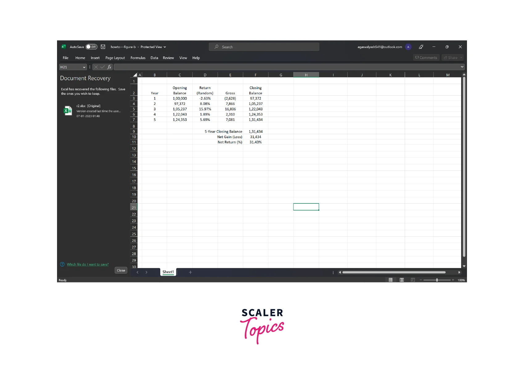
Step 1: Adding Random Data In a static Excel spreadsheet model, the inputs to the model would typically be fixed values. In a Monte Carlo simulation, these fixed values are replaced with probability distributions that represent the uncertainty associated with each input. For example, instead of a fixed expected return for an investment, we might use a normal distribution with a mean and standard deviation that reflect the historical variability of the returns.
-
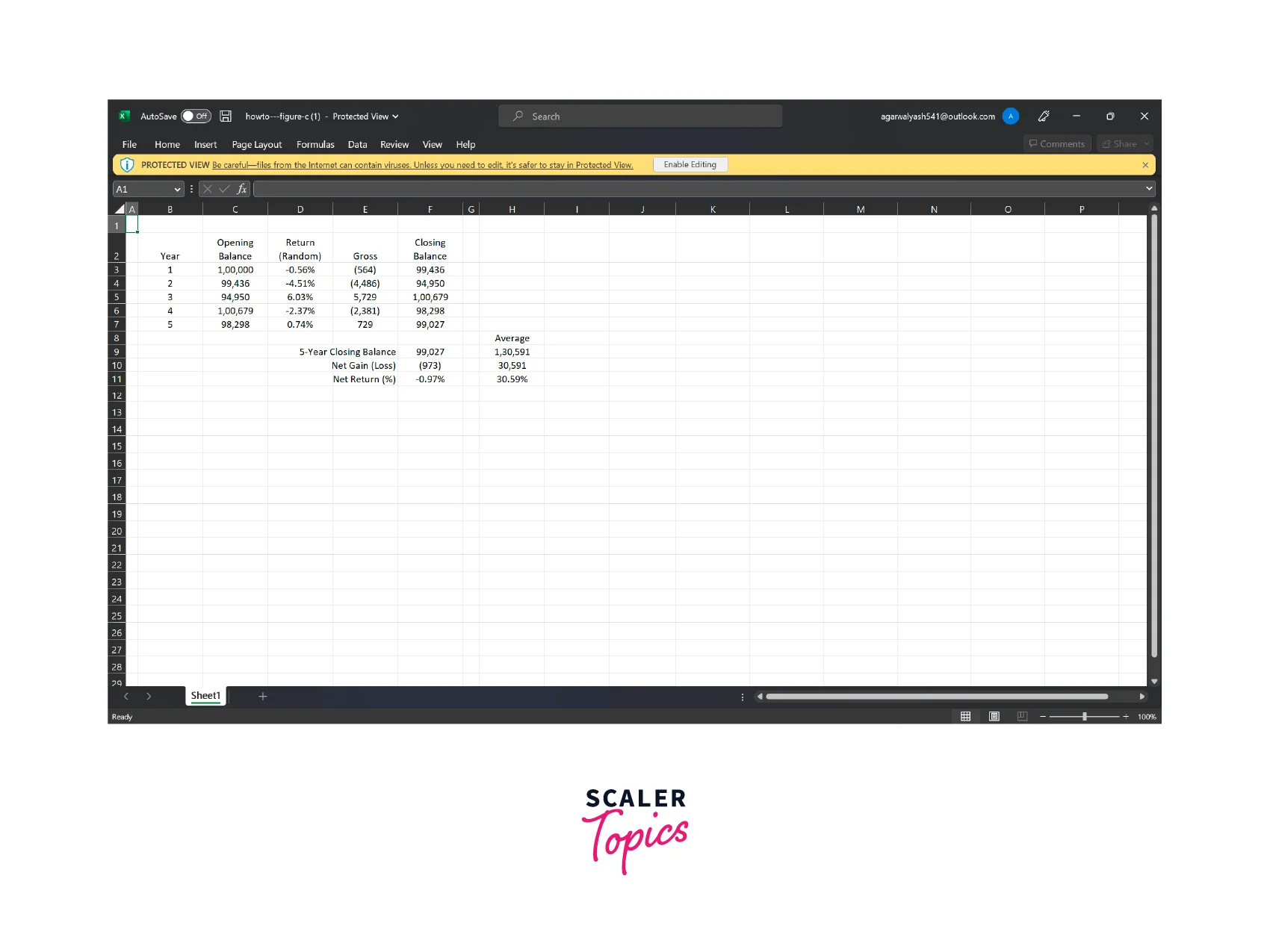
Step 2: Running a Monte Carlo Simulation Once the probability distributions for the inputs have been defined, the Monte Carlo simulation can be run. This involves generating random samples from each of the input distributions and using these samples to calculate the output of the model. In the Investment Portfolio Model, this might involve calculating the expected return, variance, and Sharpe ratio of the portfolio for each random sample.
-
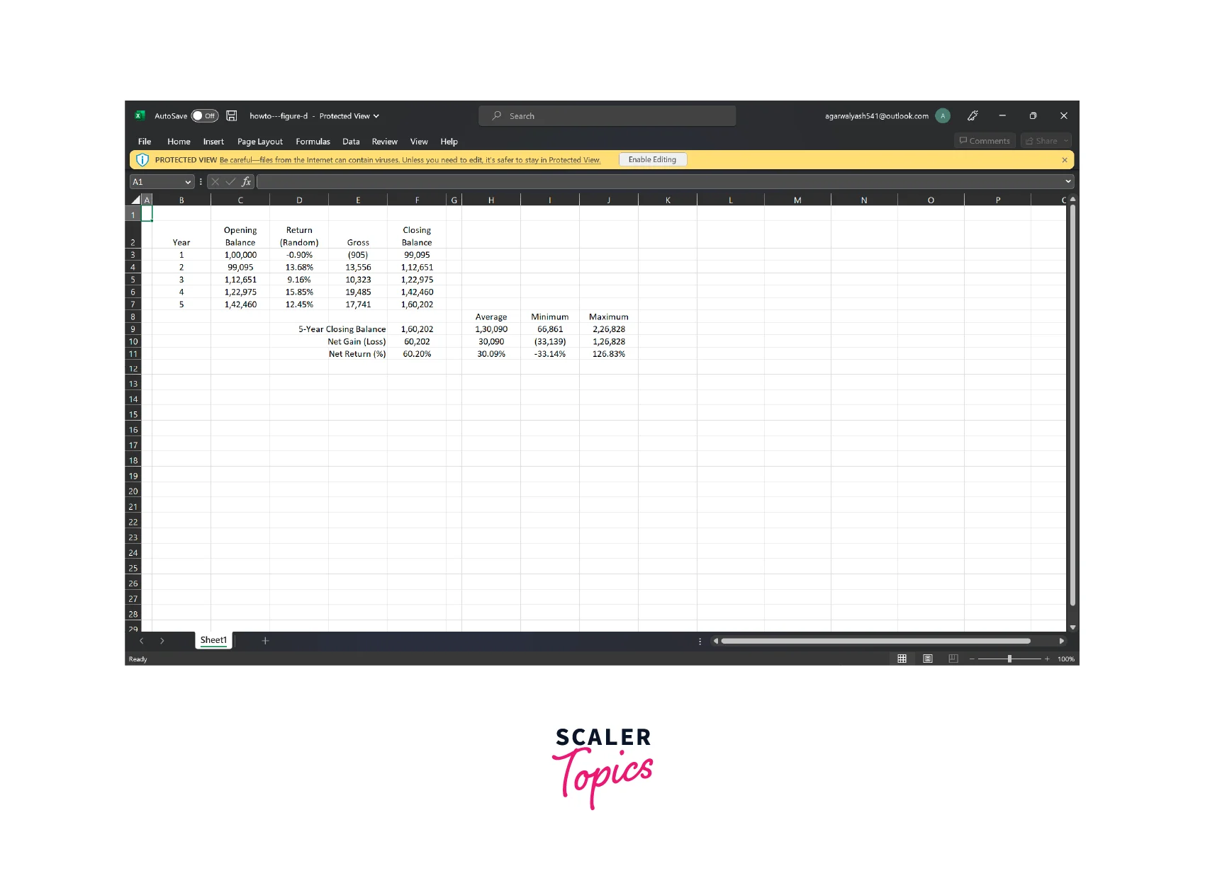
Step 3: Analyzing Data After running the Monte Carlo simulation, the output data can be analyzed to gain insights into the behavior of the system. This might involve calculating summary statistics such as the mean, median, and standard deviation of the output, or generating histograms and scatterplots to visualize the distribution of the output.
-
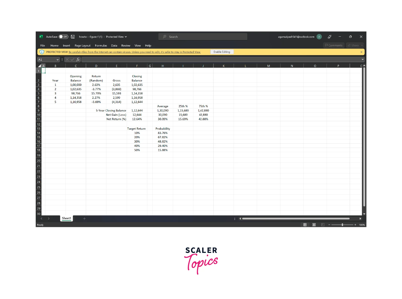
Step 4: Determining Confidence Levels One of the key benefits of Monte Carlo simulation is that it allows us to estimate confidence levels for the output of the model. By generating a large number of random samples and calculating the output for each sample, we can estimate the probability of the output falling within a certain range. For example, we might be interested in the probability of the portfolio generating a positive return over a given period. By analyzing the output data, we can estimate the probability of this occurring and use this information to inform our decision-making.
Converting a static Excel spreadsheet model into a Monte Carlo simulation involves replacing fixed input values with probability distributions, generating random samples from these distributions, analyzing the output data, and estimating confidence levels for the output. The Investment Portfolio Model provides a useful example of how Monte Carlo simulation can be applied in the context of financial modeling.
Conclusion
- Monte Carlo simulation is a powerful technique used to model and analyze complex systems by generating multiple random samples and analyzing the resulting output data.
- It allows us to estimate the probability of outcomes and helps in making informed decisions by taking into account the uncertainty associated with a system.
- Monte Carlo simulation is widely used in finance, engineering, and many other fields where the behavior of a system is uncertain or difficult to predict.
- This technique can be used to convert a static Excel spreadsheet model into a Monte Carlo simulation by replacing fixed input values with probability distributions, generating random samples from these distributions, analyzing the output data, and estimating confidence levels for the output.
- The results of the Monte Carlo simulation can provide valuable insights into the behavior of a system and help in identifying key drivers of performance.
- Monte Carlo simulation also has its limitations, such as the assumption of independent variables and the need for large sample sizes to generate accurate results.
- Overall, Monte Carlo simulation is a powerful tool for decision-making and should be considered when dealing with complex systems with uncertain outcomes.