Normal Distribution in R
Overview
The Normal distribution in R is a fundamental concept in statistics, often referred to as the Gaussian distribution. It is a symmetric bell-shaped probability distribution that describes many real-world phenomena. In this article, we will delve into the world of normal distribution in R, exploring its significance and how to work with it using various functions.
What is Normal Distribution in R?
The Normal distribution in R refers to the capability of the R programming language to handle and manipulate data that follows a normal distribution pattern. The normal distribution, often known as the Gaussian distribution, is a widely used probability distribution that is characterized by its symmetric bell-shaped curve. It is a fundamental concept in statistics and finds application in various fields including finance, natural sciences, and social sciences.
Key Functions for Working with Normal Distribution in R
Here are the four primary functions that empower R users to work with the normal distribution seamlessly:
-
dnorm() - Probability Density Calculation:
This function computes the probability density at a given point in a normal distribution. Probability density represents the likelihood of a specific value occurring within a given interval.
Syntax: dnorm(x, mean = 0, sd = 1)
Parameters:
- x: The point at which the density will be calculated.
- mean: The mean of the distribution (default is 0).
- sd: The standard deviation of the distribution (default is 1).
-
pnorm() - Cumulative Distribution Calculation:
The pnorm() function calculates the cumulative distribution function (CDF) value for a specified point in a normal distribution. The CDF represents the probability of observing a value less than or equal to the given point.
Syntax: pnorm(q, mean = 0, sd = 1)
Parameters:
- q: The point for which the CDF value will be calculated.
- mean: The mean of the distribution (default is 0).
- sd: The standard deviation of the distribution (default is 1).
-
qnorm() - Quantile Calculation:
With the qnorm() function, you can find the quantile value corresponding to a given probability in a normal distribution. Quantiles help identify values below which a certain percentage of observations fall.
Syntax: qnorm(p, mean = 0, sd = 1)
Parameters:
- p: The probability for which the quantile value will be determined.
- mean: The mean of the distribution (default is 0).
- sd: The standard deviation of the distribution (default is 1).
-
rnorm() - Random Data Generation
This function generates random numbers that adhere to a normal distribution pattern. It's a valuable tool for creating synthetic datasets or conducting simulations.
Syntax: rnorm(n, mean = 0, sd = 1)
Parameters:
- n: The number of random values to be generated.
- mean: The mean of the distribution (default is 0).
- sd: The standard deviation of the distribution (default is 1).
Functions to Generate Normal Distribution in R
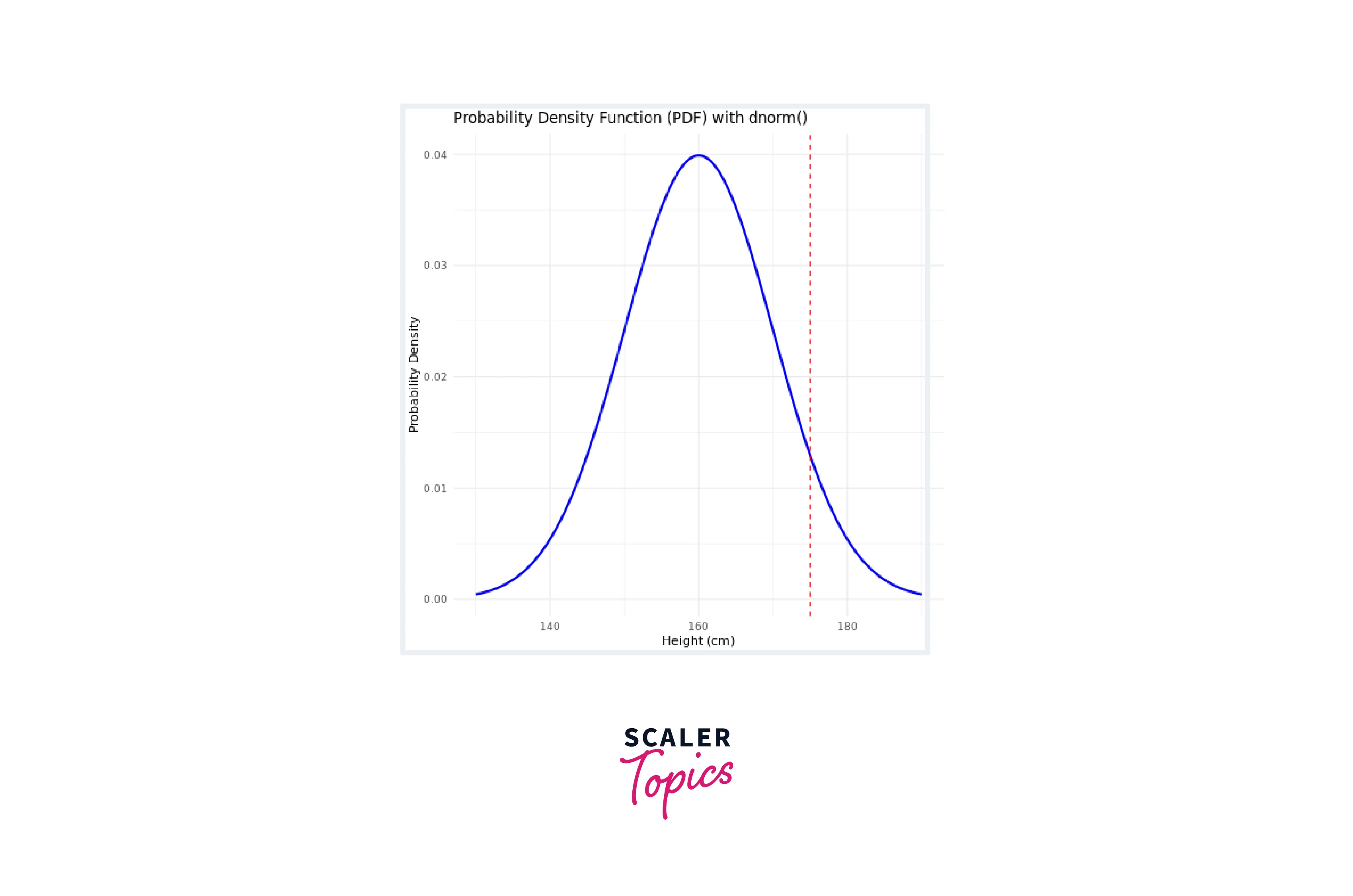
dnorm()
The dnorm() function calculates the probability density at a specific point in a normal distribution. This is essential for understanding the likelihood of observing a particular value in the distribution.
Syntax: dnorm(x, mean = 0, sd = 1)
Example:
Consider a dataset representing the heights of individuals in a population. Let's calculate the probability density for a height of 175 cm, assuming a mean height of 160 cm and a standard deviation of 10 cm.
Output:
pnorm()
The pnorm() function computes the cumulative distribution function (CDF) value for a specific point in a normal distribution. This helps in determining the probability of observing a value less than or equal to the given point.
Syntax: pnorm(q, mean = 0, sd = 1)
Example: Using the same height dataset, let's calculate the cumulative distribution for a height of 170 cm.
Output:
qnorm()
The qnorm() function allows you to find the quantile value corresponding to a given probability in a normal distribution. This is useful when you need to determine the value below which a certain percentage of observations fall.
Syntax: qnorm(p, mean = 0, sd = 1)
Example:
Continuing with the height dataset, let's find the height below which 80% of individuals fall.
Output:
rnorm()
The rnorm() function is used to generate random numbers that follow a normal distribution pattern. This is valuable for creating synthetic datasets or conducting simulations.
Syntax: rnorm(n, mean = 0, sd = 1)
Example: Let's generate a sample of 10 random heights from a normal distribution with a mean of 170 cm and a standard deviation of 5 cm.
Output:
Conclusion
- The normal distribution in R is a fundamental concept, applicable across diverse fields. R's dedicated functions empower users to seamlessly integrate its principles into their analyses.
- The four core functions — dnorm(), pnorm(), qnorm(), and rnorm() — enable precise probability density calculations, cumulative distribution evaluations, quantile determinations, and random data generation, respectively.
- Applying these functions to real data offers valuable insights. They enable assessing the likelihood of values, understanding cumulative probabilities, determining quantile thresholds, and simulating scenarios, aiding robust data analysis.
- Beyond its mathematical nature, the normal distribution becomes a universal ally. It assists researchers, analysts, and decision-makers in comprehending data trends and facilitating informed choices.