Optimal Binary Search Tree

Overview

A binary search tree is a tree in which the nodes in the left subtree are smaller than the root node, while the nodes in the right subtree are greater than the root node. When we talk about binary search trees, the searching concept comes first. The cost of searching for a node in the tree plays a very important role. Our purpose is to reduce the cost of searching, and that can only be done by an optimal binary search tree.

The optimal binary search tree (Optimal BST) is also known as a weight-balanced search tree. It is a binary search tree that provides the shortest possible search time or expected search time. An optimal binary search tree is helpful in dictionary search.

Let’s take an example for better understanding:

Let’s assume that we have the following keys in our tree: 15, 25, 35, 45, 55, 65, 75

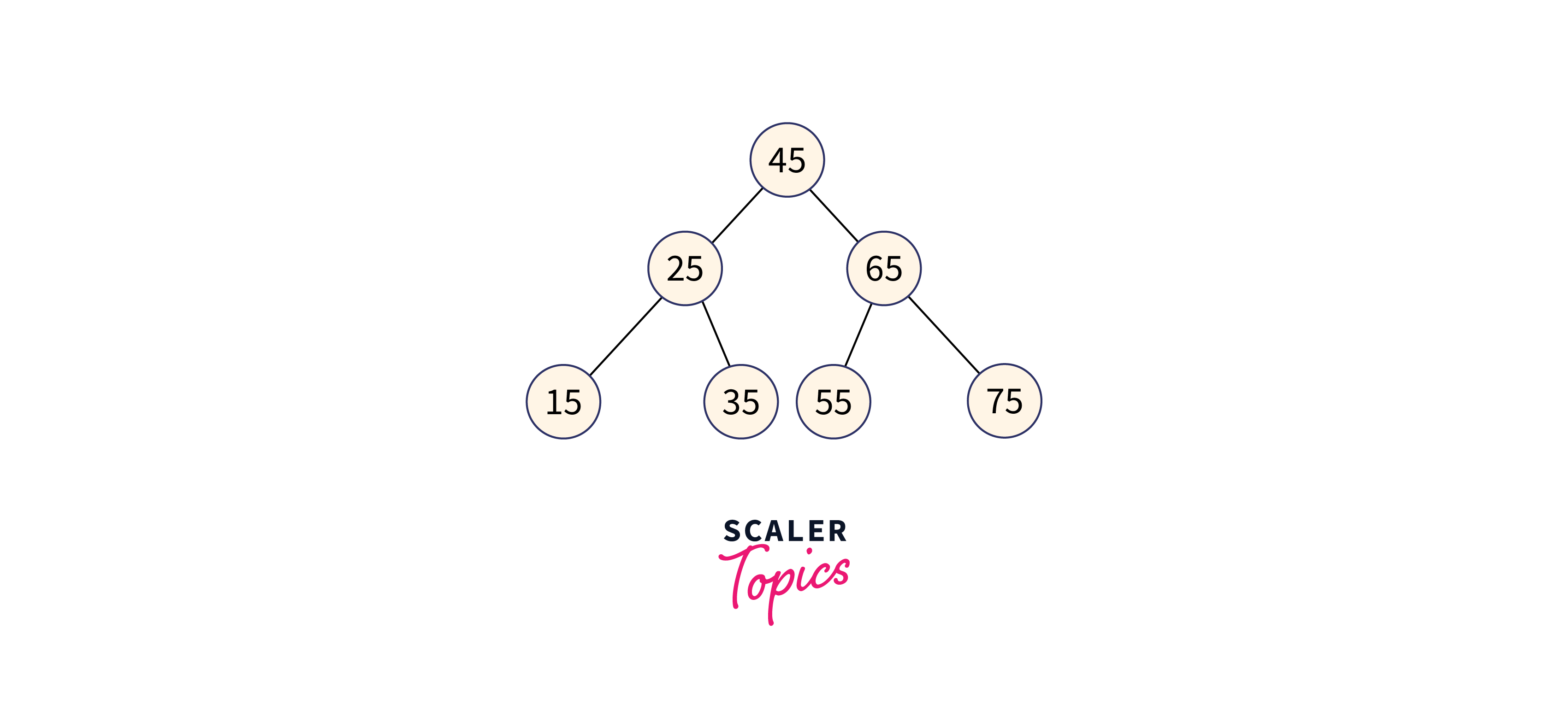
The maximum time required to search a node in a binary search tree is equal to the minimum height of the tree i.e. logn.

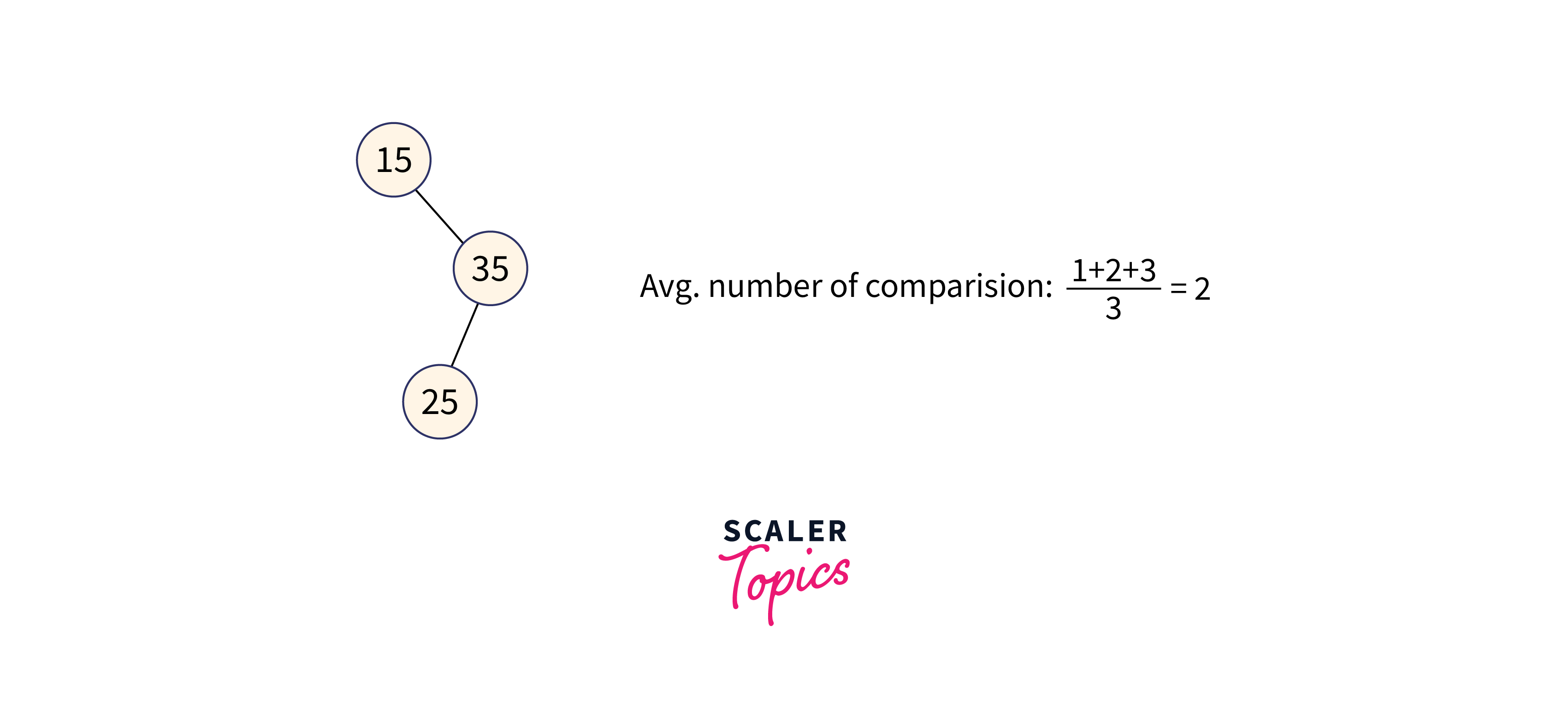
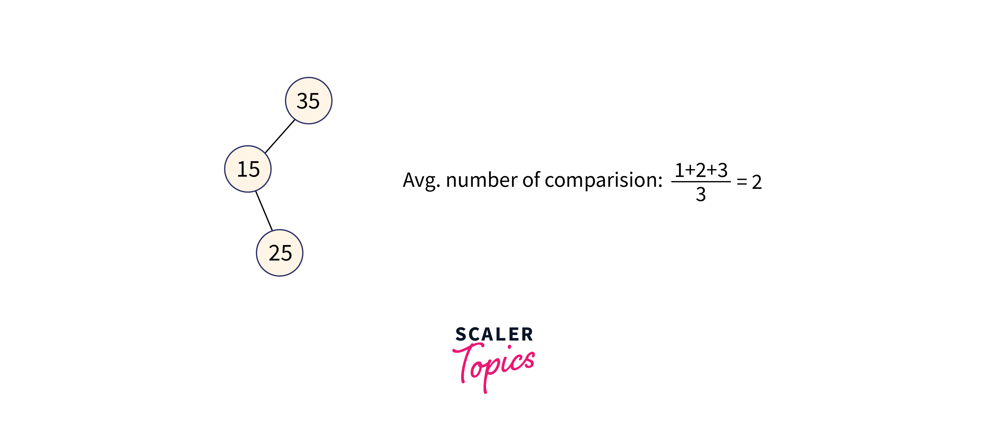
If we have keys: 15, 25, 35, then see how many BST can be formed. We will use the formula given below:

= ${}^{2n}C_{n} \over n+1$

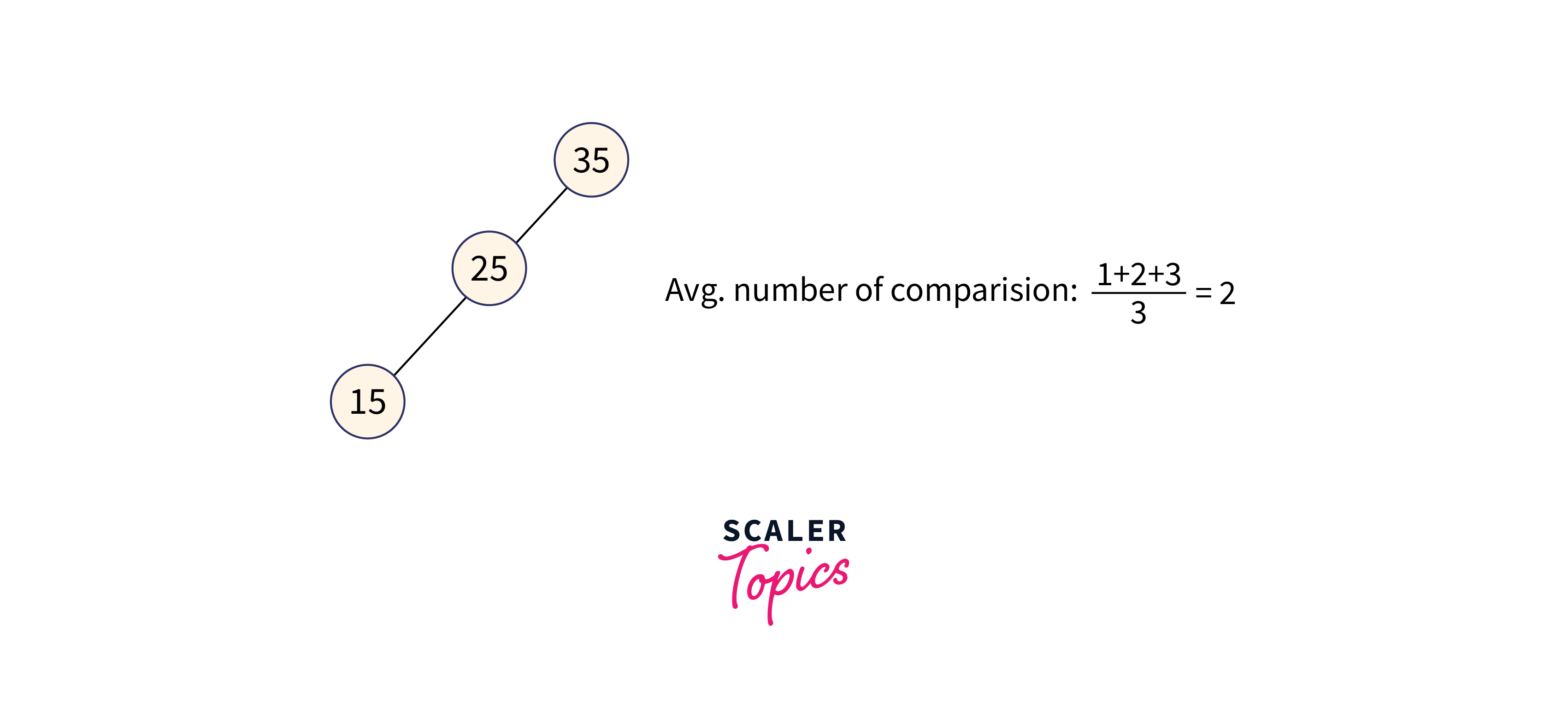
So we can see that 5 trees will be formed as shown in the figure given below.

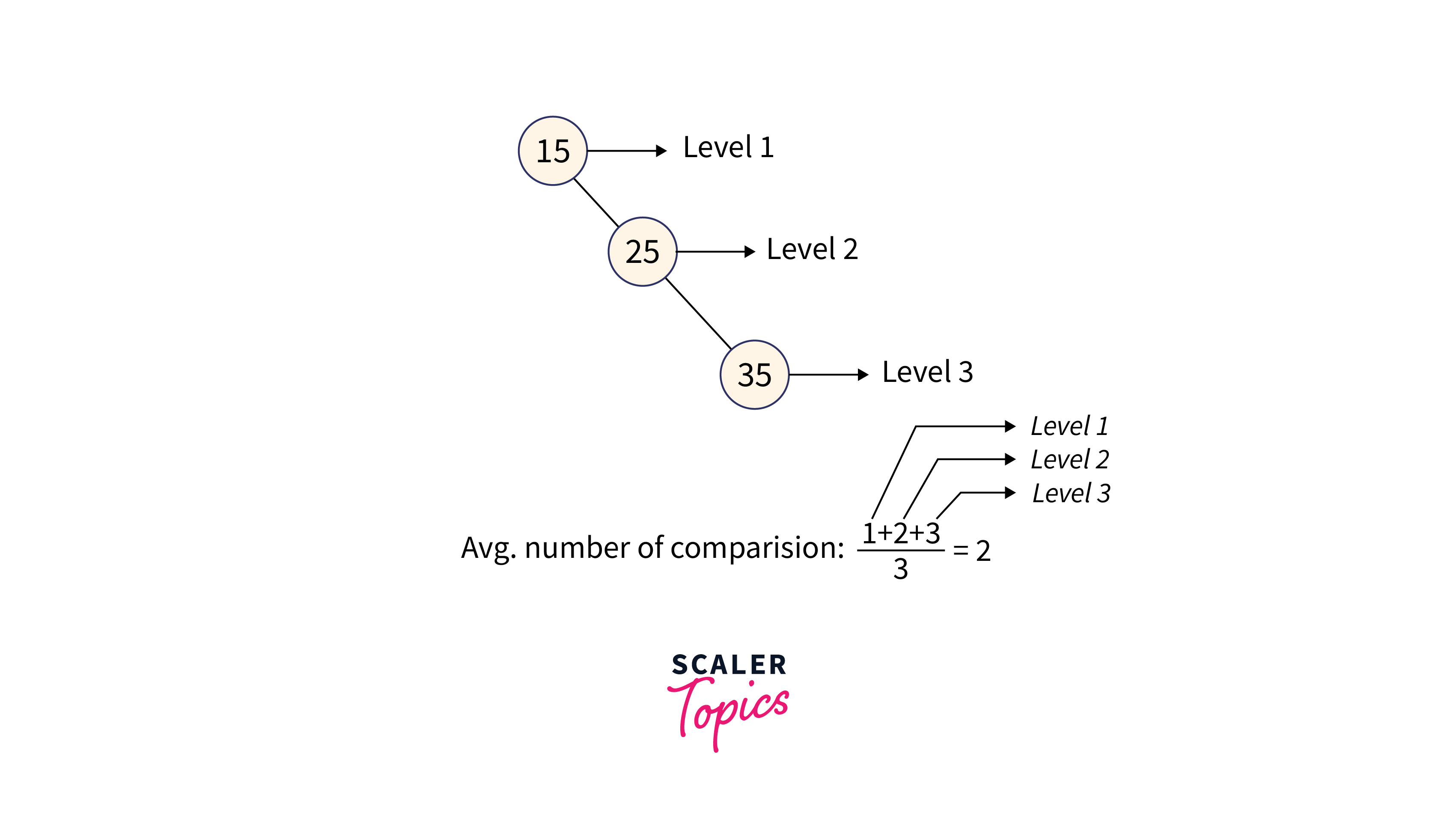
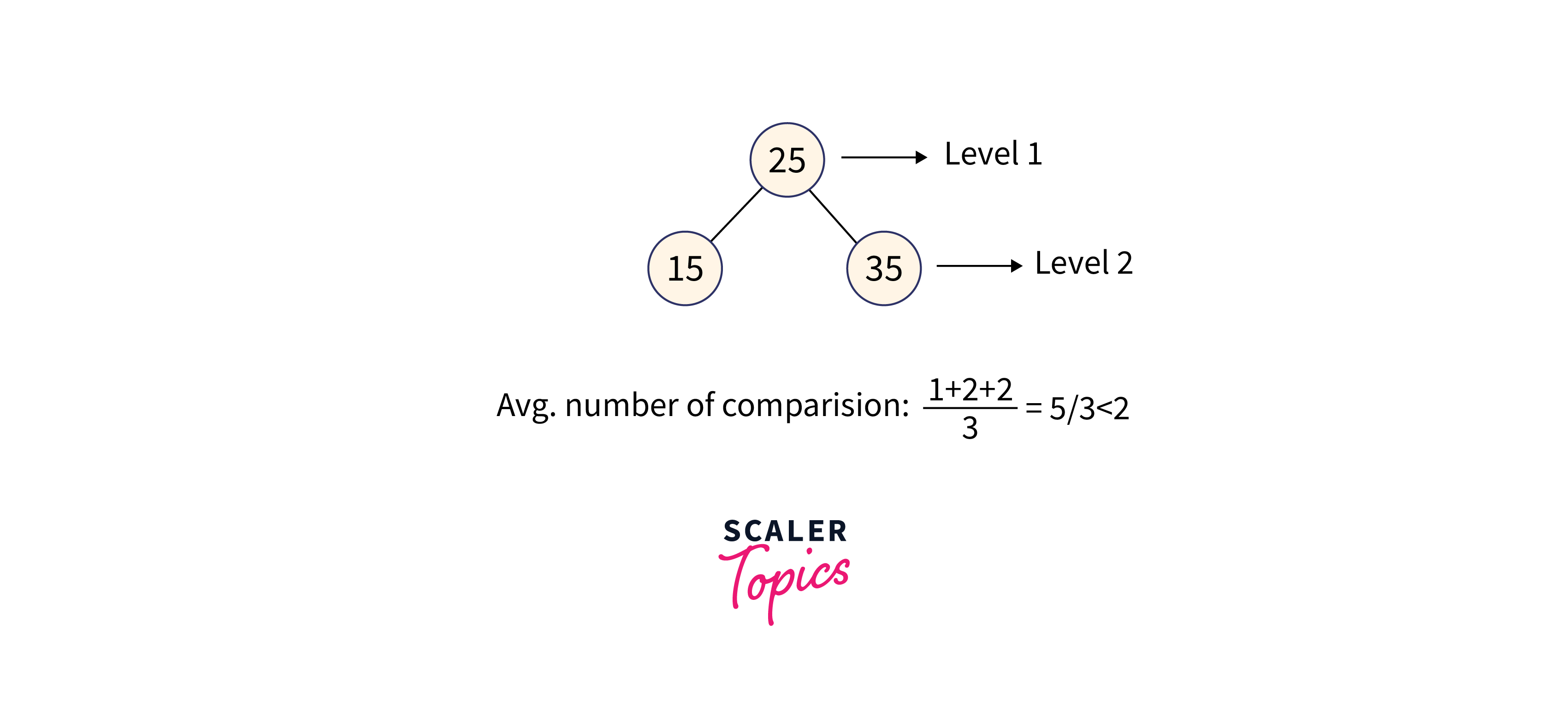
Avg. number of comparisons: $\frac{1+2+3}{3}=2$

Avg no of comparisons $=\frac{1+2+3}{3}=2$

\text { Avg. number of Comparisons: } \frac{1+2+2}{3}=5 / 3<2 \text {. }

Avg no of comparisons $=\frac{1+2+3}{3}=2$

In the third case, the total number of comparisons is less as compared to others because the height of the tree is less. So we can say that it’s a balanced binary search tree.

Mathematical Formulation

The keys in the OBST are in the sorted order ki……..kj, where 1<=i<=j<=n.
The subtree containing keys ki….kj, has leaves with dummy keys di-1……dj.
Suppose kr is the root of the subtree containing keys ki………kj. So the left subtree of the root kr has the keys ki……kr-1 and the right subtree contains keys kr+1 to kj.
Let’s assume e[i, j] represents the expected cost of searching OBST. With n keys, our aim is to find and minimize e[1, n].
The base case occurs when j = i – 1, because we just have the dummy key di-1 for this case. For this case, the expected search cost is e [i, j] = e [i, i - 1] = qi-1.
For the case, j ≥ i, we have to select any key kr from ki…kj as a root of the tree.
With kr as a root key and sub tree ki…kj, the sum of probability is defined as:

$\mathrm{w(i,j)} = \sum_{n=i}^{j} p_m + \sum_{m=i-1}^{j} q_m$

Recursive formula for forming a OBST is given below:

e[i, j] = \begin{cases} q_{i-1} & \quad \text{if $j = i-1$}\\ min\{e[i, r-1] + e[r+1, j] + w(i, j)\} \\ i \leq r \leq j & \quad \text{if ${i \leq j}$} \end{cases}

Algorithm

First, we construct a BST from a set of n distinct keys <k1, k2, k3,... kn >. Here we assume, the probability of accessing a key Ki is pi. Some dummy keys (d0, d1, d2, ... dn) are added as some searches may be performed for the values which are not present in the Key set K. We assume, for each dummy key, di probability of access is qi.

Algorithm for finding optimal tree for sorted, distinct keys ki…kj:

For each possible root, kr for i≤r≤ji≤r≤j
Make optimal subtree for ki,…,kr−1.
Make optimal subtree for kr+1,…,kj.
Select a root that gives the best total tree.

Complexity Analysis of Optimal Binary Search Tree

We can easily derive the complexity of the above algorithm. We can see that it has three nested loops. The innermost loop statements run in Q(1) time.

\begin{aligned} T(n) & =\sum_{m=1}^n \sum_{i=1}^{n-m+1} \sum_{j=i}^{n-1+1} \theta(1) \\ & =\sum_{m=1}^n \sum_{i=1}^{n-m+1} n=\sum_{m=1}^n n^2 \\ & =\theta\left(n^3\right) \end{aligned}

The above algorithm runs in Cubic time.

Example

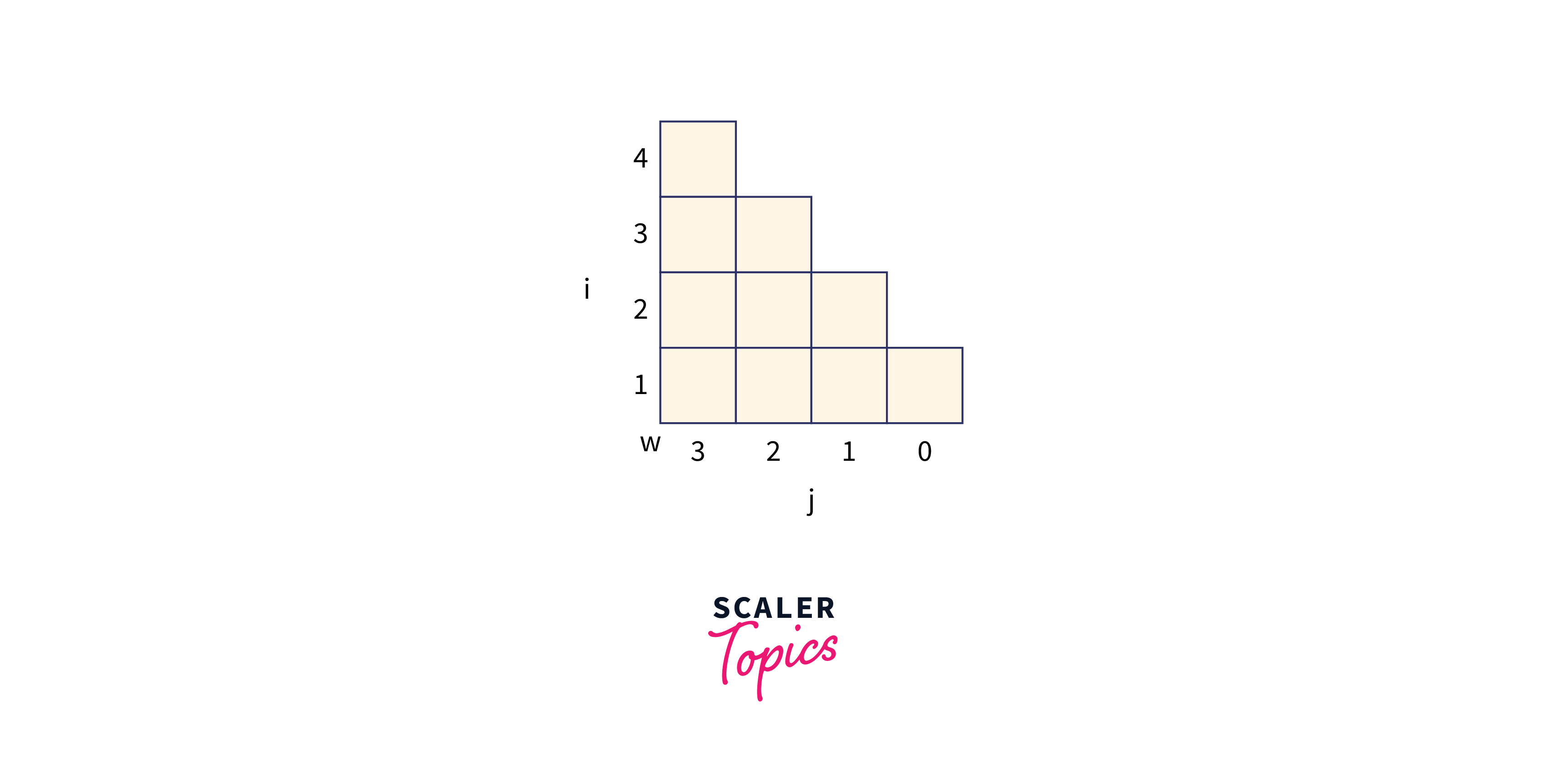
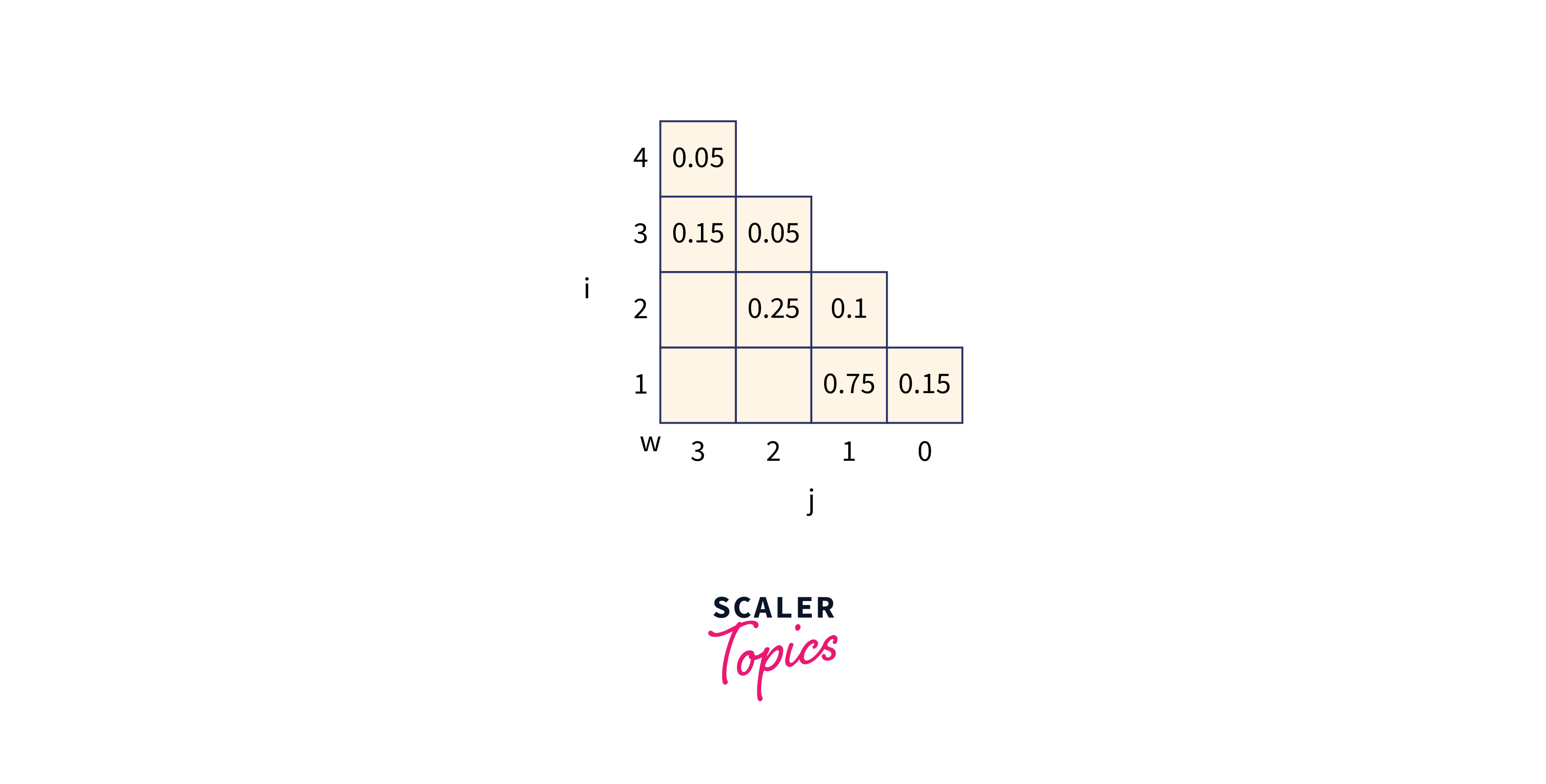
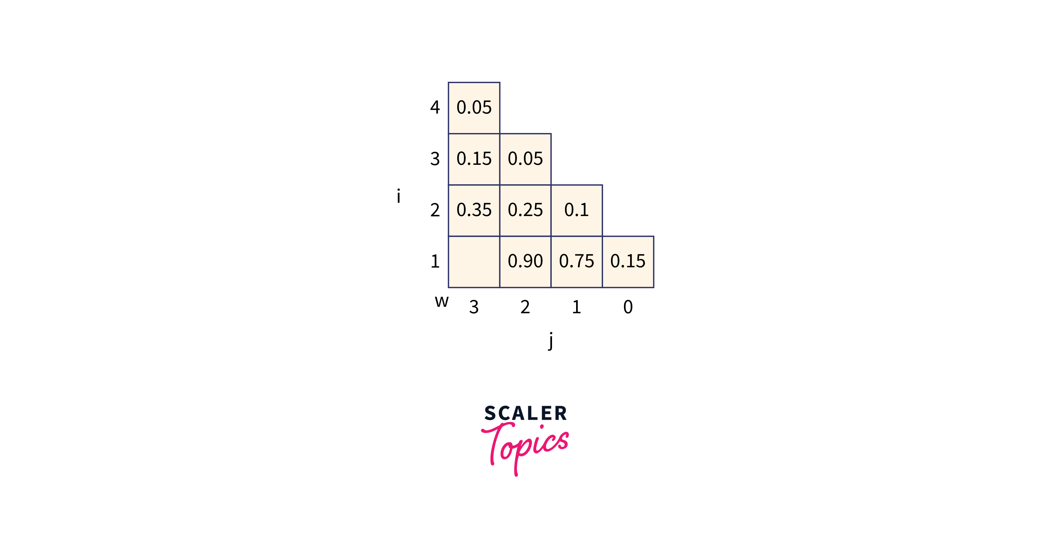
Let p (1 : 3) = (0.5, 0.1, 0.05) q(0 : 3) = (0.15, 0.1, 0.05, 0.05) Compute and construct OBST for above values using Dynamic approach.

Recursive Formula to solve $O B S T$ :

e[i, j]= \begin{cases}q_{i-1} & \text { if } j=i-1 \\ \min \{e[j, r-1]+e[r+1, j]+w(i, j) & \\ i \leqslant r \leqslant j\} & \text { if } i \leqslant j\end{cases}

where,

\omega(i, j)=\sum_{m=1}^j p_m+\sum_{m=i-1}^j q_m

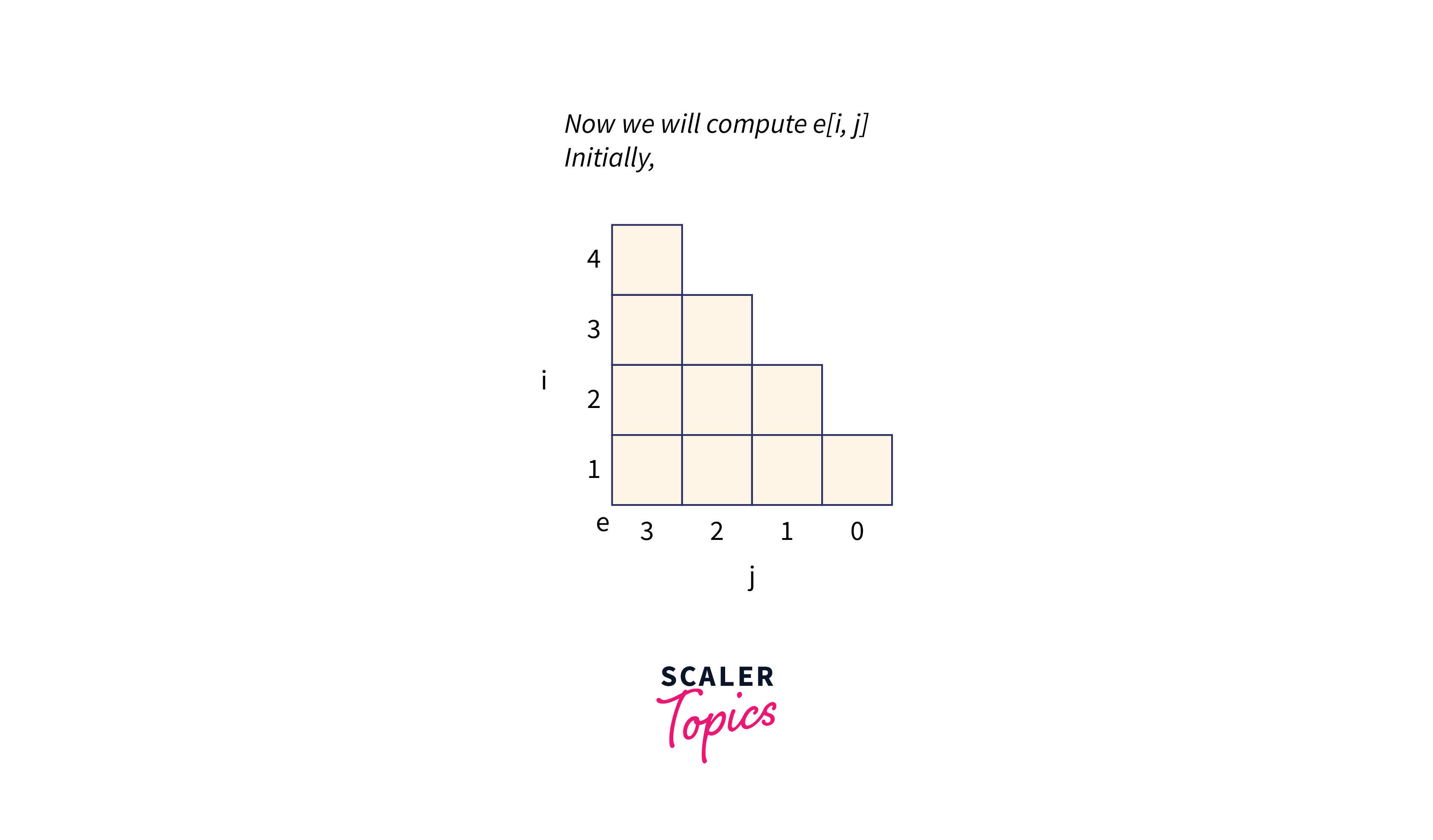
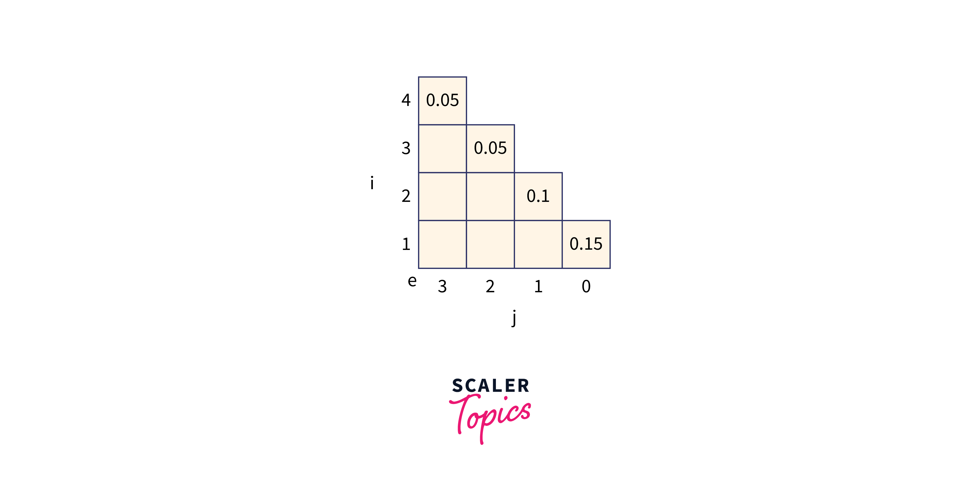
mitially,

w[1,0]=\sum_{m=1}^0 p_m+\sum_{m=0}^0 q_m=q_0=0.15

$\begin{aligned} \omega[2,1] & =\sum_{m=2}^1 p_m+\sum_{m=1}^1 q_m=q_1=0.1 \\ \omega[3,2] & =\sum_{m=3}^2 p_m+\sum_{m=2}^2 q_m=q_2=0.05 \\ \omega[4,3] & =\sum_{m=4}^3 p_m+\sum_{m=3}^3 q_m=q_3=0.05\end{aligned}$

$\begin{aligned} & w[1,1]=\sum_{m=1}^1 p_m+\sum_{m=0}^1 q_m=p_1+q_0+q_1 \\ & =0.5 \text { +0. } 25=0.75 \\ & w[2,2]=\sum_{m=2}^2 p_m+\sum_{m=1}^2 q_m=p_2+q_1+q_2 \\ & =0.1+0.15=0.25 \\ & w[3,3]=\sum_{m=3}^3 p_m+\sum_{m=2}^3 q_m=p_3+q_2+q_3 \\ & =0.05+0.10=0.15 \\ & \end{aligned}$

$\begin{aligned} \omega[1,2] & =\sum_{m=1}^2 p_m+\sum_{m=0}^2 q_m \\ & =\left(p_1+p_2\right)+\left(q_0+q_1+q_2\right) \\ & =0.6+0.3=0.90 \\ \omega[2,3] & =\sum_{m=2}^3 p_m+\sum_{m=1}^3-q_m, \\ & =\left(p_2+p_3\right)+\left(q_1+q_2+q_3\right) \\ & =0.15+0.2=0.35\end{aligned}$

$\begin{aligned} w[1,3] & =\sum_{m=1}^3 p_m+\sum_{m=0}^3 q_m \\ & =\left(p_1+p_2+p_3\right)+\left(q_0+q_1+q_2+q_3\right) \\ & =0.65+0.35=1\end{aligned}$

$\begin{aligned} & e[1,0]=q_0=0.15 \quad(\because j=i-1) \\ & e[2,1]=q_1=0.1 \quad(\because j=i-1) \\ & e[3,2]=q_2=0.05(\because j=i-1) \\ & e[4,3]=q_3=0.05 \quad(\because j=i-1)\end{aligned}$

$\begin{aligned} e[1,1]= & \min \{e[1,0]+e[\{, 1]+w(1,1)\} \\ = & \min \{0.15+0.1+0.75\}=1.0 \\ e[2,2]= & \min \{e[2,1]+e[3,2]+w(2,2)\} \\ & =\min \{0.1+0.05+0.25\}=0.4 \\ e[3,3]= & \min \{e[3,2]+e[4,3]+w(3,3)\} \\ = & \min (0.05+0.05+0.15)=0.25\end{aligned}$

$\begin{aligned} e[1,2] & =\min \left\{\begin{array}{l}e[1,0]+e[2,2]+w[1,2] \\ e[1,1]+e[3,2]+w[1,2]\end{array}\right\} \\ & =\min \left\{\begin{array}{l}0.15+0.4+0.50 \\ 1.6+0.05+0.90\end{array}\right\} \\ & =\min \left\{\begin{array}{l}1.45 \\ 1.95\end{array}\right\}=1.45 \\ e[2,3] & =\min \left\{\begin{array}{l}e[2,1]+e[3.3]+w(2,3) \\ e[2,2] \pm e[4,3]+w(2,3)\end{array}\right\} \\ & =\min \left\{\begin{array}{l}0.1+0.25+0.35 \\ 0.4+0.05+0.35\end{array}\right\} \\ & =\min \left\{\begin{array}{l}0.90 \\ 0.80\end{array}\right\}=0.8\end{aligned}$

$\begin{aligned} e[1,3] & =\min \left\{\begin{array}{l}e[1,0]+e[2,3]+\omega(1,3) \\ e[1,1]+e[3,3]+\omega(1,3) \\ e[1,2]+e[4,3]+\omega(1,3)\end{array}\right\} \\ & =\min \left\{\begin{array}{l}0.15+0.80+1.0 \\ 1.0+0.25+1.0 \\ 1.45+0.05+1.0\end{array}\right\} \\ & =\min \left\{\begin{array}{l}1.95 \\ 2.25 \\ 2.5\end{array}\right\}=1.95\end{aligned}$

Types

Optimal BST is divided into two types:

Static Optimality:

In the static optimality problem, the tree can’t be modified after it has been constructed. In this instance, a specific configuration of the tree's nodes offers the shortest predicted search time for the specified access probabilities.

Dynamic Optimality:

In the dynamic optimality problem, the tree can be modified at any time by tree rotations. In the tree, the cursor is pointing at the root node so that it can move or perform modifications. The cursor in this case visits each node in the target access sequence sequentially thanks to some low-cost sequence of these operations.

How to Solve Optimal Binary Search Tree (with Implementation Code and Complexity Analysis)

We have given a sorted array of keys, which consists of keys to be searched and a frequency array of frequency counts.

We have to construct a binary search tree such that the total cost of all the searches is as small as possible. First we will calculate the cost, but how to calculate the cost?

"Cost is the level of that node multiplied by frequency."

Let's take an example to understand it properly:

Now, we see the recusrive and dynamic programming code to find the cost of optimal BST.

Using Recursive Approach

\begin{aligned} & \text { Optcost }(i, j)=\sum_{k=i}^j \text { freq }[k]+\min _{r=i}^j[\operatorname{opt} \cos t(i, r-1)+ \\ & \text { opt cost }(r+1, j)] \\ & \end{aligned}

The plan is to try each node as root one at a time (r varies from i to j in the second term). Making the rth node the root allows us to determine the optimal cost from i to r-1 and r+1 to j recursively.

The frequencies from i to j are summed (see first term in the above formula).

C++

Output:

Java

Output:

Python

Output:

Complexity Analysis:

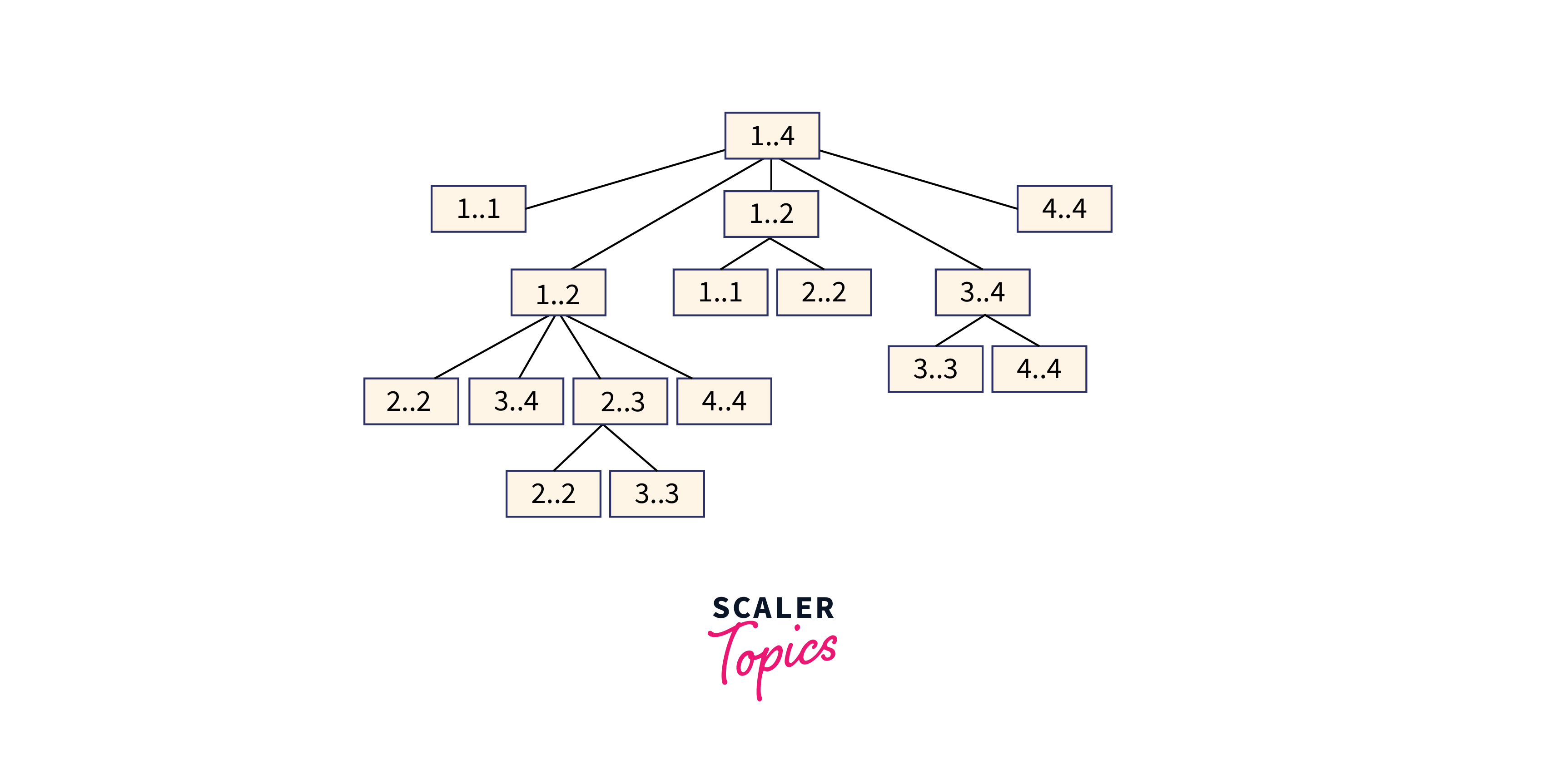
The basic recursive technique described above has exponential time complexity. It should be noted that the above function repeatedly computes the same subproblems. In the recursion tree for frequency [1...4], we can see that several subproblems are being repeated. Since the same problem is repeated again and again, this problem has the overlapping subproblem property.

Using Dynamic Programming

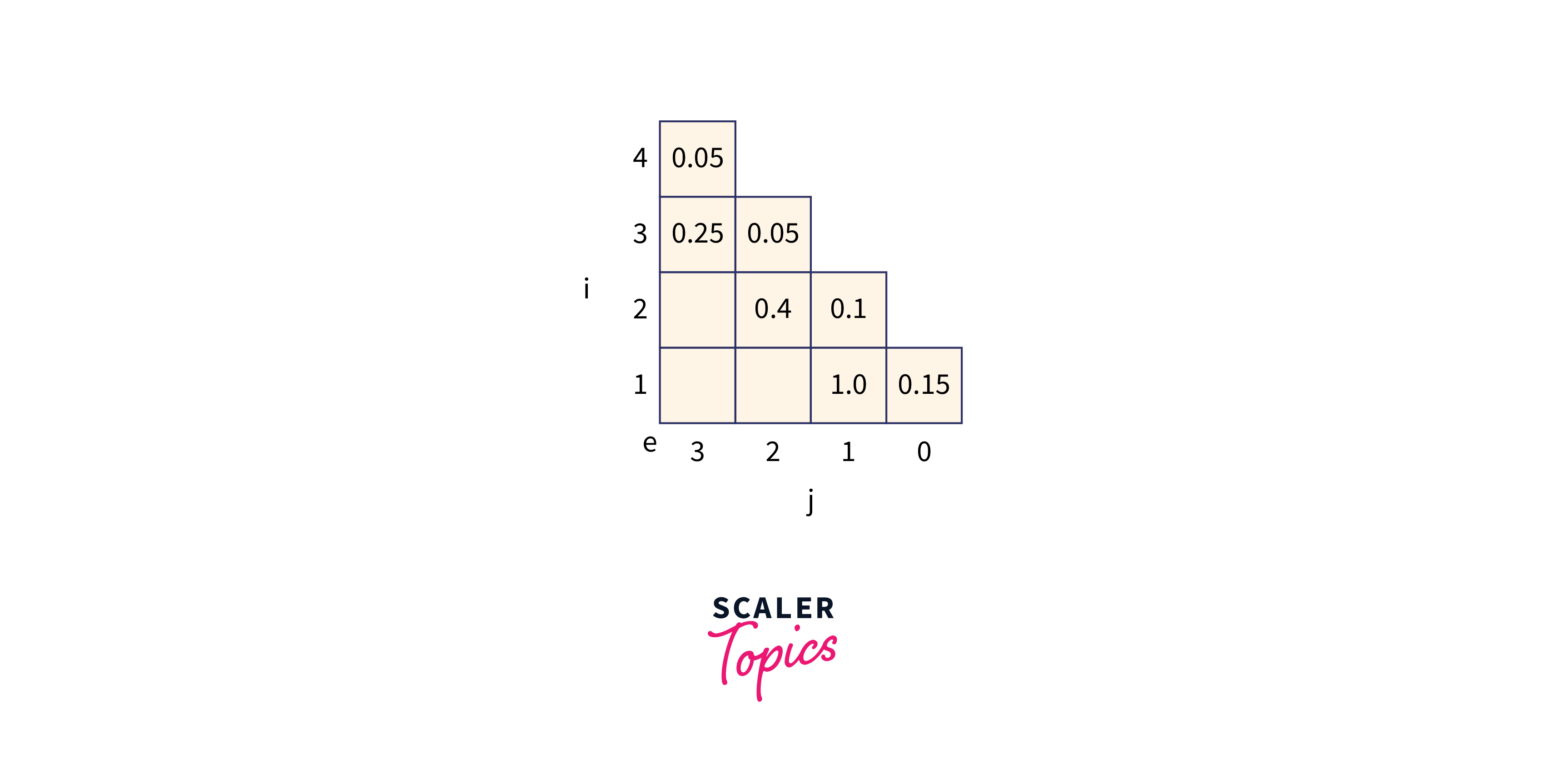
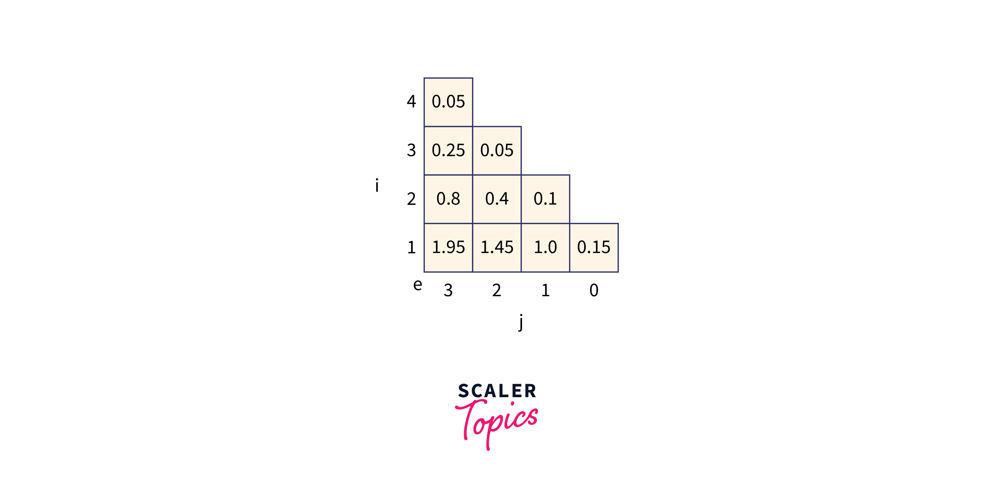
We use an auxiliary array cost[n][n] to store the solutions of subproblems. cost[0][n-1] will hold the final result. The challenge is that all diagonal values must be filled first, then the values that lie on the line just above the diagonal. Or in a simple way, we need to first fill in all the cost[i][i] values, then all the cost[i][i+1] values, and finally all the cost[i][i+2] values.

C++

Output:

Java

Output:

Python

Output:

Complexity Analysis:

Time complexity:

The above solution has an $O(n^4)$ time complexity. By precalculating the sum of frequencies rather than continuously calling the add() function, the time complexity can be easily reduced to $O(n^3)$ .

Space Complexity:

The above solution has an $O(n^2)$ space complexity since we are making a 2D array.

Conclusion

Let's conclude our topic on optimal binary search trees by mentioning some of the most important points:

An optimal binary search tree is a binary search tree that provides the shortest possible search time or expected search time and it is also known as a weight-balanced search tree.
The cost of searching for a node in the tree plays a vital role, and it is decided by the frequency and key value of the node.
Optimal BST is divided into two types: Static Optimality and Dynamic Optimality.
The basic recursive technique has exponential time complexity. It should be noted that the optCost function repeatedly computes the same subproblems.
In dynamic programming approach, by precalculating the sum of frequencies rather than continuously calling the add() function, the time complexity can be easily reduced to $O(n^3)$ .