Pivot Tables in Excel

What is a Pivot Table in Excel?

One of the fundamental tools for data analysis is the pivot table. Many significant business concerns can be quickly solved with pivot table in excel.

Pivot table in excel are created, among other things, to convey information. We want to bolster our narrative with transparent and understandable data.

Pivot Tables can be considered a form of visual storytelling, even if they are merely tables and lack actual graphics.

Data that is recorded in a table can be summarised, sorted, reorganized, grouped, counted, totaled, or averaged using a pivot table. It enables us to change rows into columns and columns into columns. Advanced calculations can be performed on them when grouping them according to any field (column).

To put it more simply, a pivot table can:

1. Arrange records, rows, and items into categories.
2. Find the minimum or maximum value, add up the value of the objects in each category, compute the average, etc.

A tool for exploring and summarising vast volumes of data, examining related totals, and presenting summary reports, an Excel pivot table can be used to:

• Present a lot of information in an approachable way.
• By using categories and subcategories, summarise the data.
• To focus on the most important details, group, sort, and conditionally format various subsets of data.
• Use "pivoting" to rotate rows to columns or columns to rows to see various summaries of the underlying data.
• The spreadsheet's total and aggregate numerical values.
• To see the specifics underlying any total, dive down and expand or collapse the data levels.
• Present your information clearly and attractively online or in printed reports.

For instance, your spreadsheet might have hundreds of entries with data on local resellers' sales:

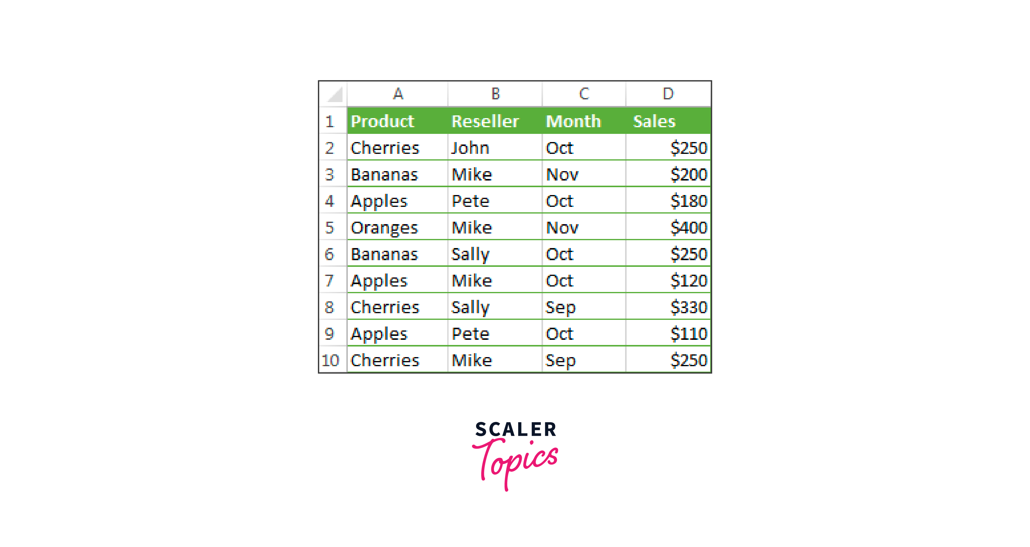
The formulas shown in the SUMIF and SUMIFS tutorials can sum up this long list of numbers by one or more conditions. However, employing a pivot table is a far more effective method to compare several facts about each figure. You may quickly and easily create a summary table that totals the data for any field with just a few mouse clicks.

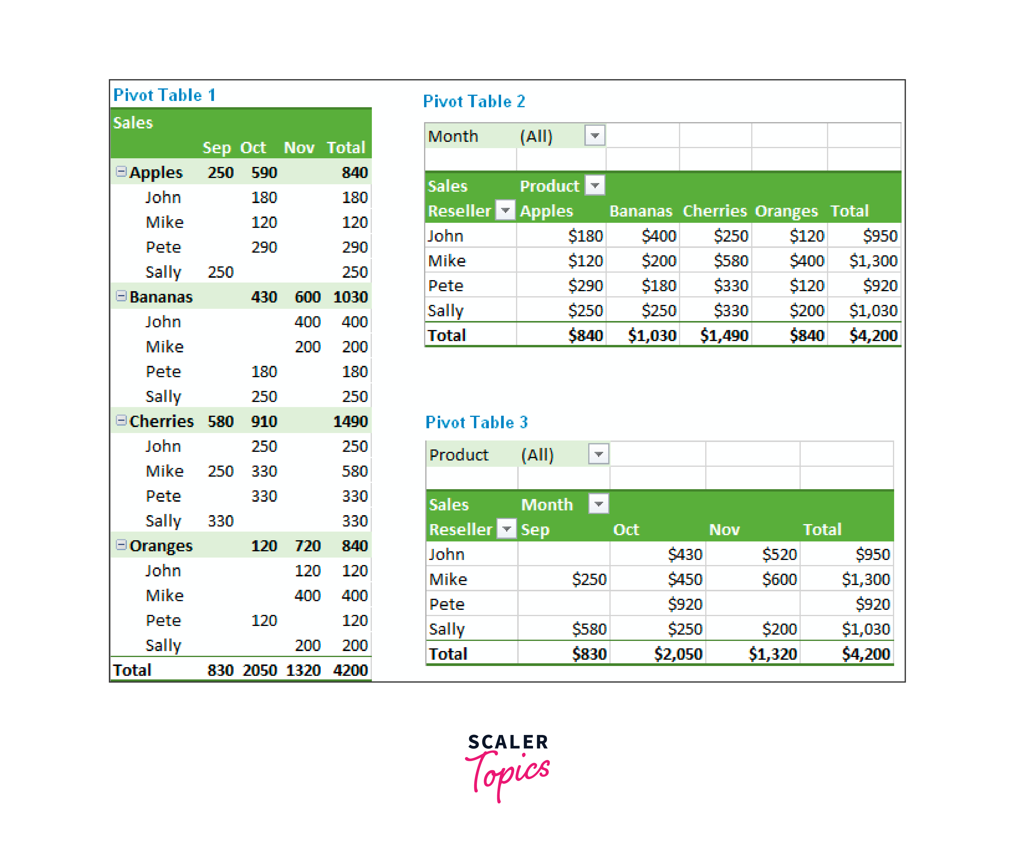
The layouts in the screenshots above are just a few options. And the instructions below demonstrate how to design your pivot table in excel version rapidly.

How to Create a Pivot Table in Excel?

Many individuals believe that constructing a pivot table is time- and labor-intensive. However, this is untrue! Microsoft has improved the technology over many years, and the summary reports in the most recent Excel versions are extraordinarily quick and user-friendly. In reality, creating your summary table only takes a few minutes. And this is how:

1. Prepare your source data

   Organize your data into rows and columns before generating a summary report, and then export your data range as an Excel Table. To do this, pick all the data and click Table on the Insert tab.

   An added benefit of using an Excel Table as the source data is that your data range becomes "dynamic". You won't have to worry about your pivot table not having the most recent data because in this context, the word "dynamic range" refers to a table that automatically expands and contracts as things are added or removed.

   Useful hints:

   • Give your columns interesting, distinctive titles; they will later serve as field names.
   • Ensure your source table has no subtotals, blank rows, columns, or empty spaces.
   • By choosing the Design tab and typing the name in the Table Name box in the worksheet's upper right corner, you can give your source table a name to make it easier to maintain.

2. Create a Pivot Table

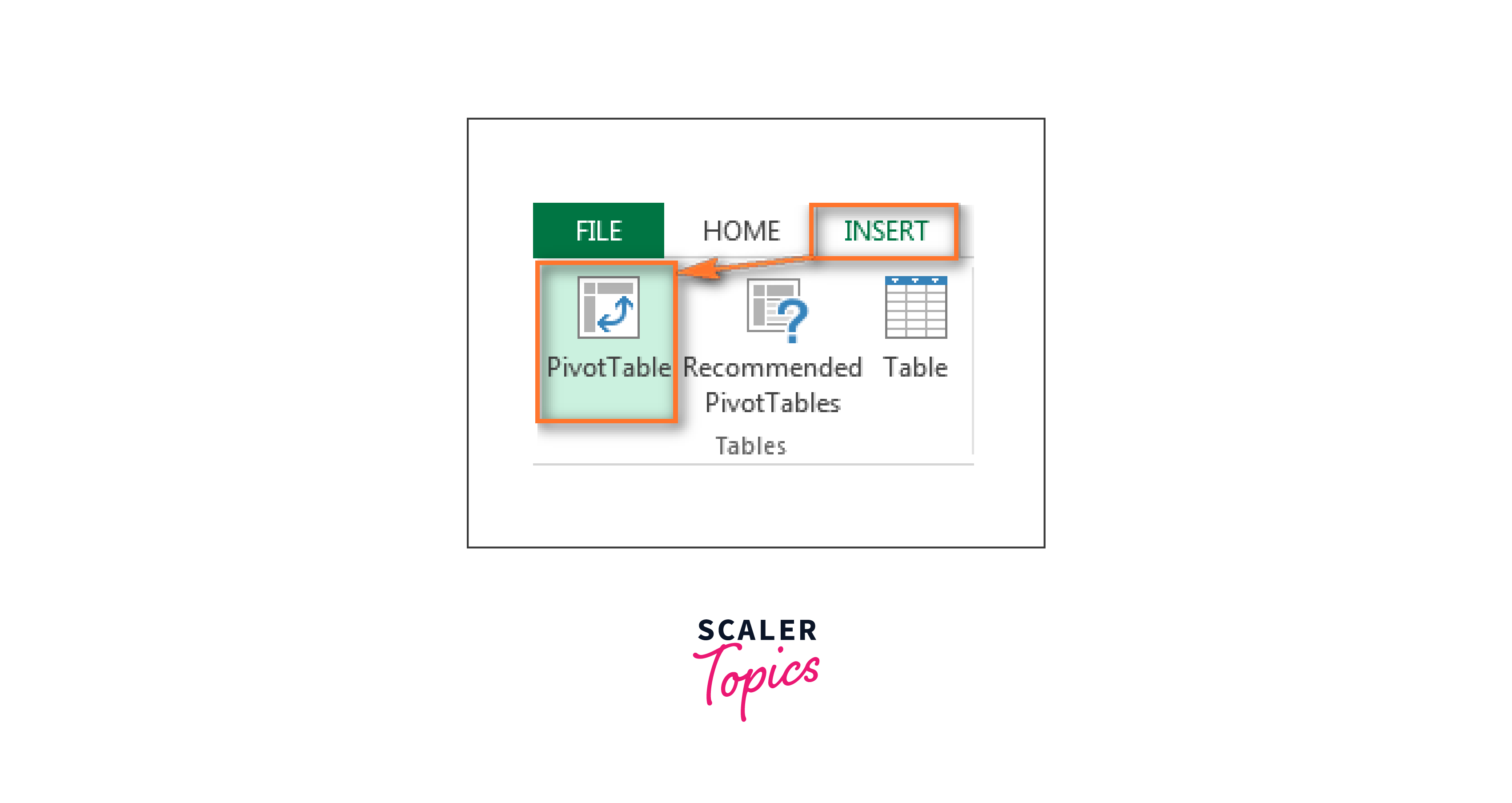
   Go to the Insert tab > Tables group > PivotTable after selecting any cell in the source data table.

   

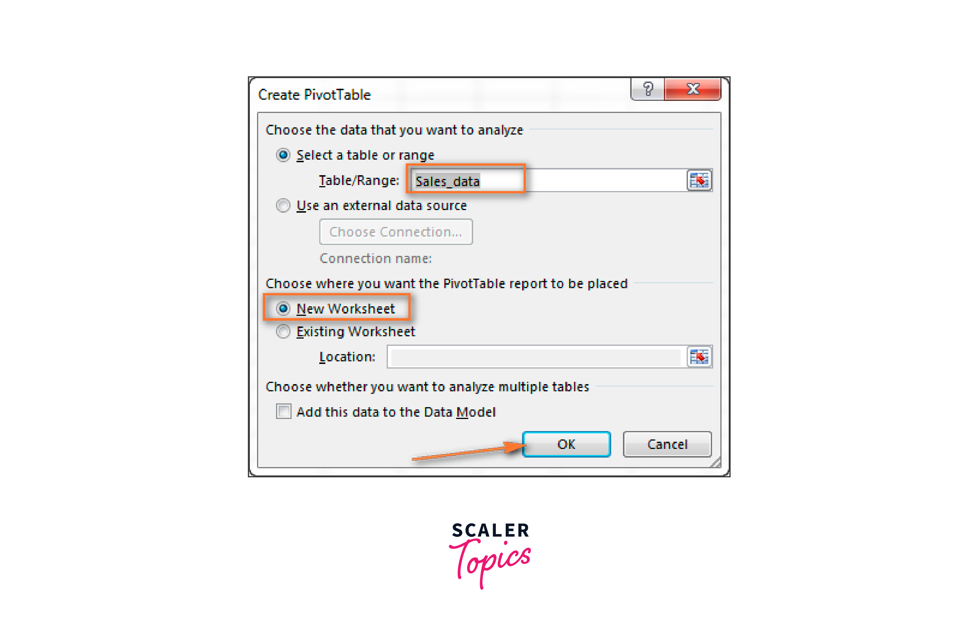
   The Create PivotTable window will open as a result. First, check that the appropriate table or cell range is highlighted in the Table/Range field. Next, decide where you want your Excel pivot table to be located:

   A table will be started in a new worksheet at cell A1 if you choose New Worksheet. When you choose an existing worksheet, your table will be inserted at the chosen spot in the worksheet. First, click the Collapse Dialogue button in the Location box. Next, select the first cell using the Collapse Dialogue button to place your table.

   

   The blank Pivot Table that is created at the desired location after clicking OK will resemble this when created:

   

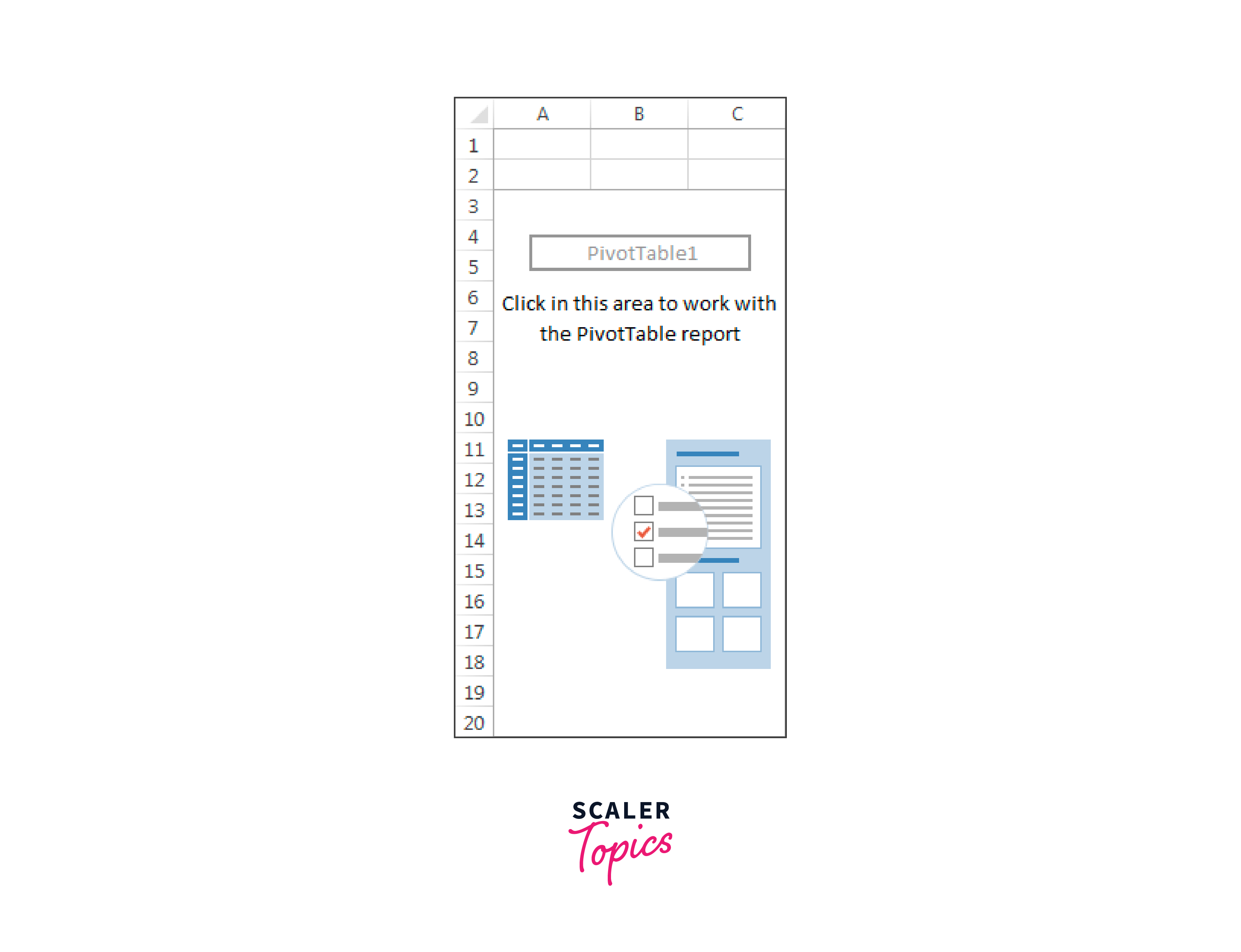
   Useful hints:

   • It usually makes sense to include a pivot table in a separate worksheet; beginners are strongly advised to do this.
   • Use the following syntax to add the workbook and worksheet names if you are building a pivot table using data from another worksheet or workbook. [workbook_name]
   • For instance, sheet_name!range [Book1.xlsx]Sheet1!$A$1:$E$20. As an alternative, press the Collapse Dialogue button. Use the mouse to pick a table or range of cells in another worksheet by clicking the Collapse Dialogue button.
   • A pivot table and pivot chart could be made at the same time. In Excel 2013 and later, select the Insert tab > Charts group, click the arrow next to the PivotChart button, and then select PivotChart & PivoTable to accomplish this. Click the arrow next to PivotTable in Excel 2010 and 2007 before selecting PivotChart.

3. Create the report's layout using Pivot Tables.

   The fields in your summary report are handled in the PivotTable Field List. It is located in the upper right corner of the worksheet and is divided into the header and body sections:

   The Field Section contains a list of the names of the fields you can use in your table. The field names correspond to the column names in your source table. The Layout Section contains the Report Filter, Column Labels, Row Labels, and Values sections. Here, you can change and arrange the fields of your table.

   

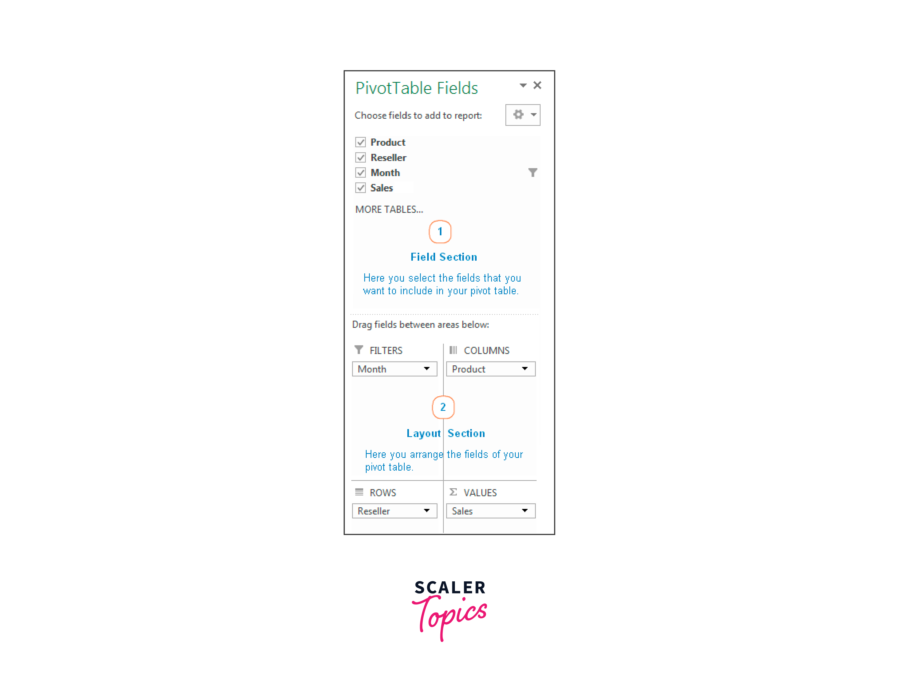
   When you change the PivotTable Field List, your table is immediately updated.

   Pivot Table field addition instructions Select the checkbox next to the field name in the Field section to add the field to the Layout section.

   

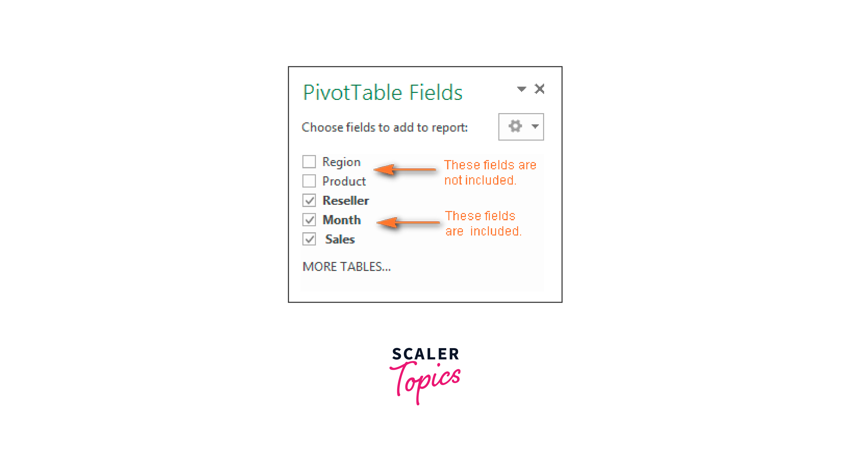
   By default, Microsoft Excel includes the following fields in the Layout section:

   Online Analytical Processing (OLAP) date and time hierarchies are added to the Column Labels area, non-numeric fields are added to the Row Labels area, numeric fields to the Values area, and all three to the Row Labels area.

   A Pivot Table field removal procedure You have two options for deleting a specific field:

   In the PivotTable pane's Field section, uncheck the box next to the field's name. Choose "Remove Field_Name" from the context menu when right-clicking the field in your pivot table.

   

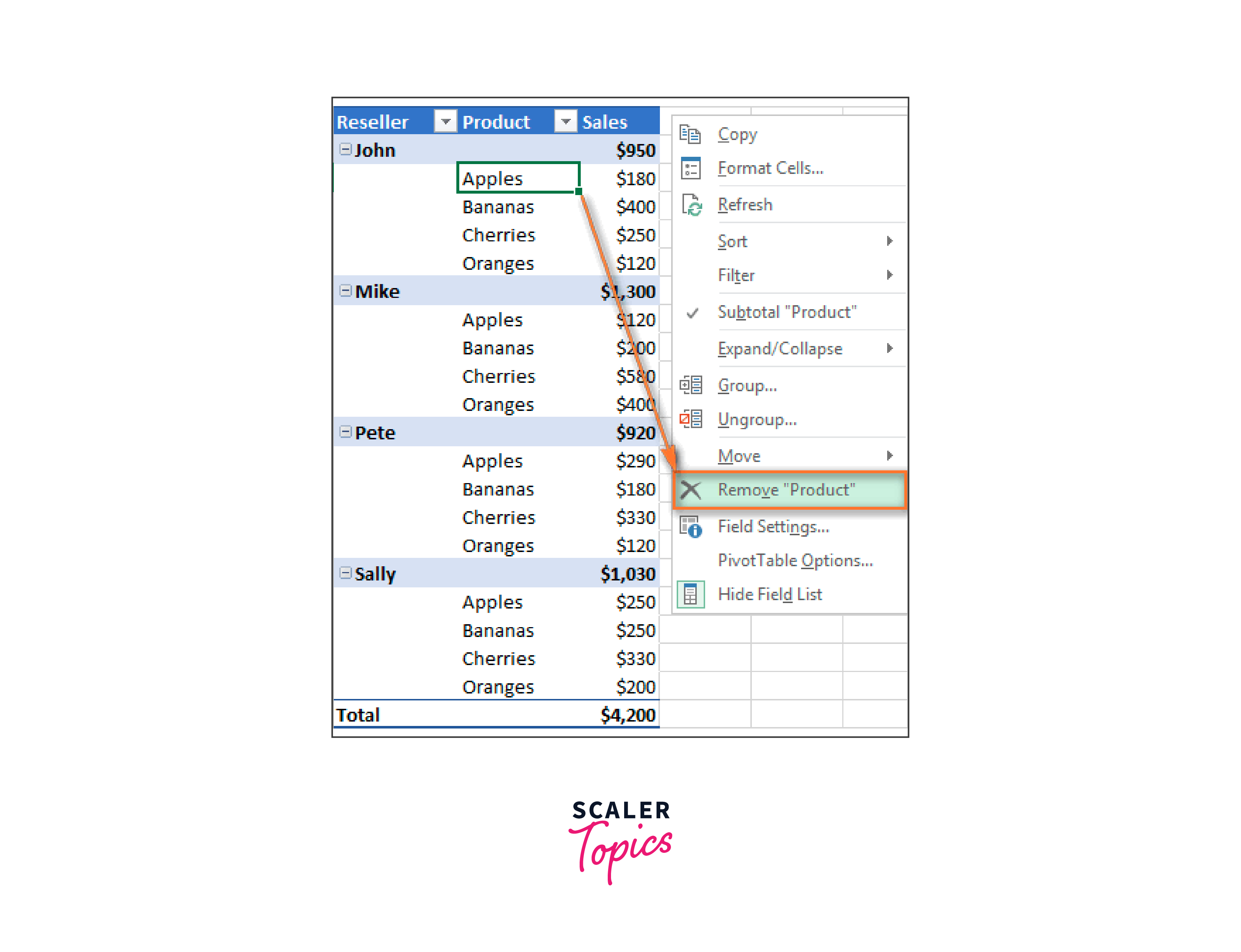
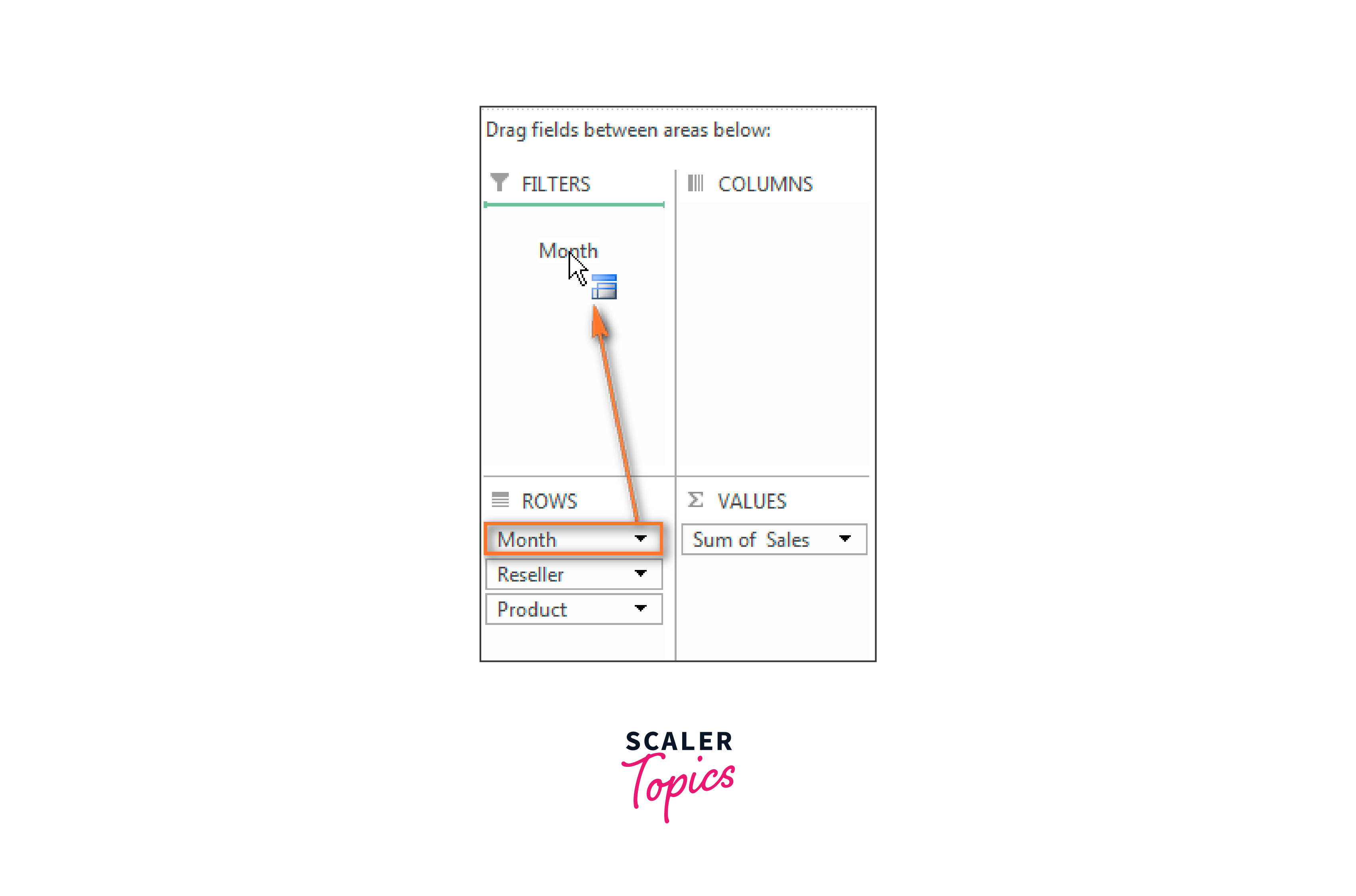
   How to set up the fields in a pivot table The fields in the Layout section can be arranged in one of three ways:

   Move fields between the four areas of the Layout section using the mouse. You may also drag the field to a different location in the Layout section by clicking and holding the field name in the Field section. The field will then move to the new location from where it is now located in the Layout section.

   

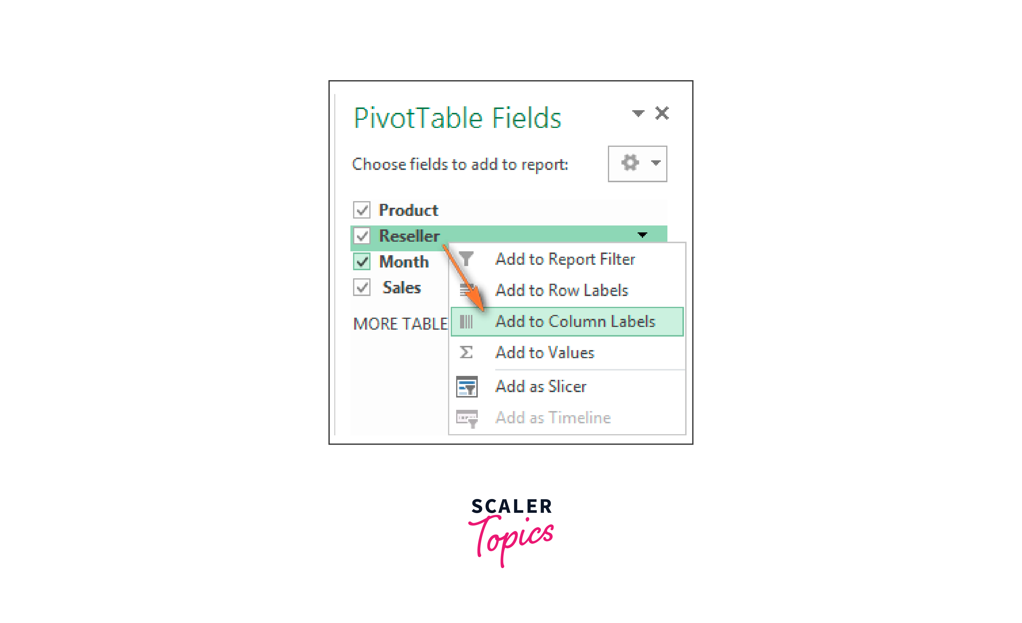
   In the Field section, right-click the field name, then choose the location where you wish to add it:

   

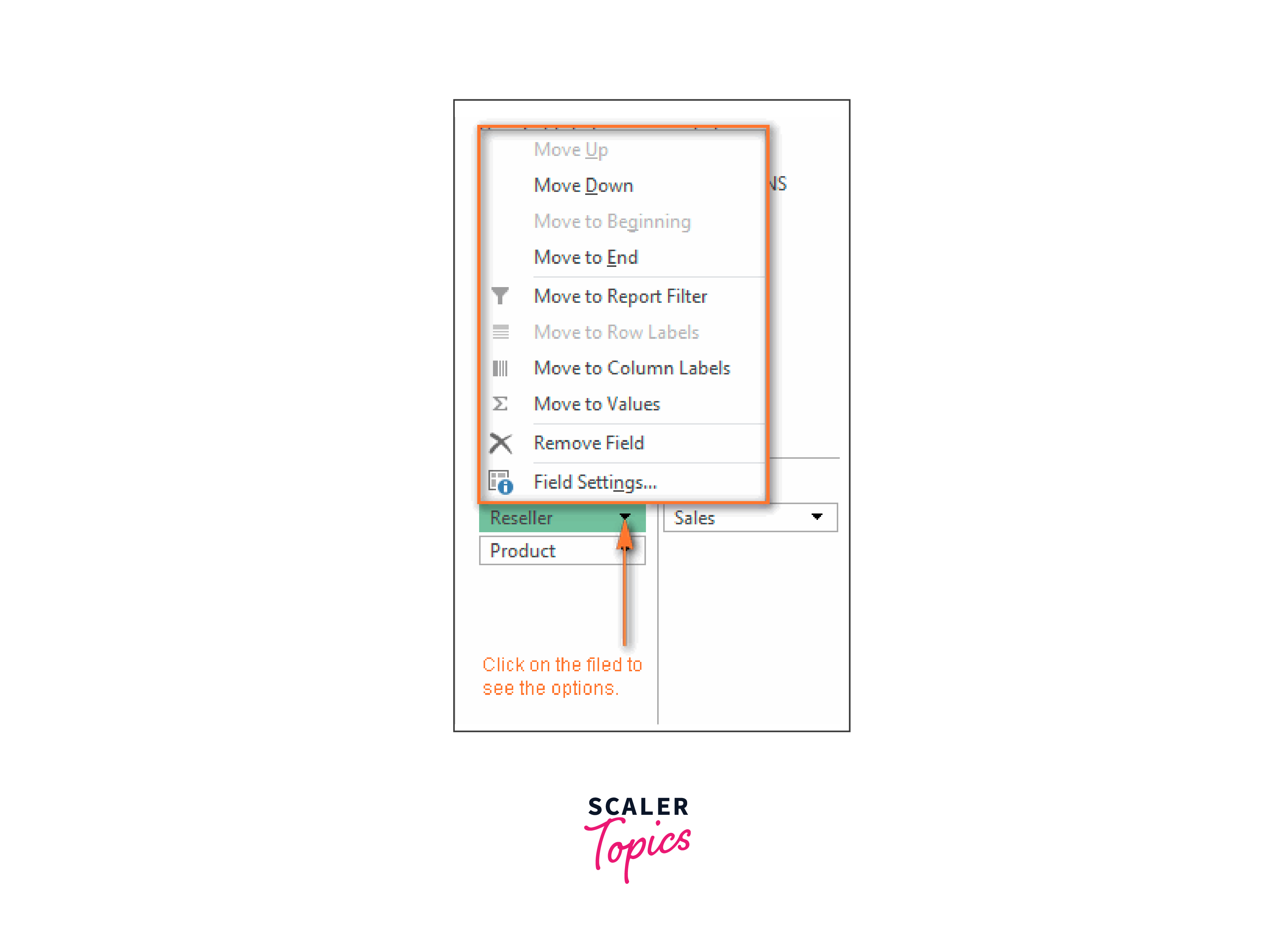
   To pick a field, click on it in the Layout section. Additionally, this

   

Drag Fields

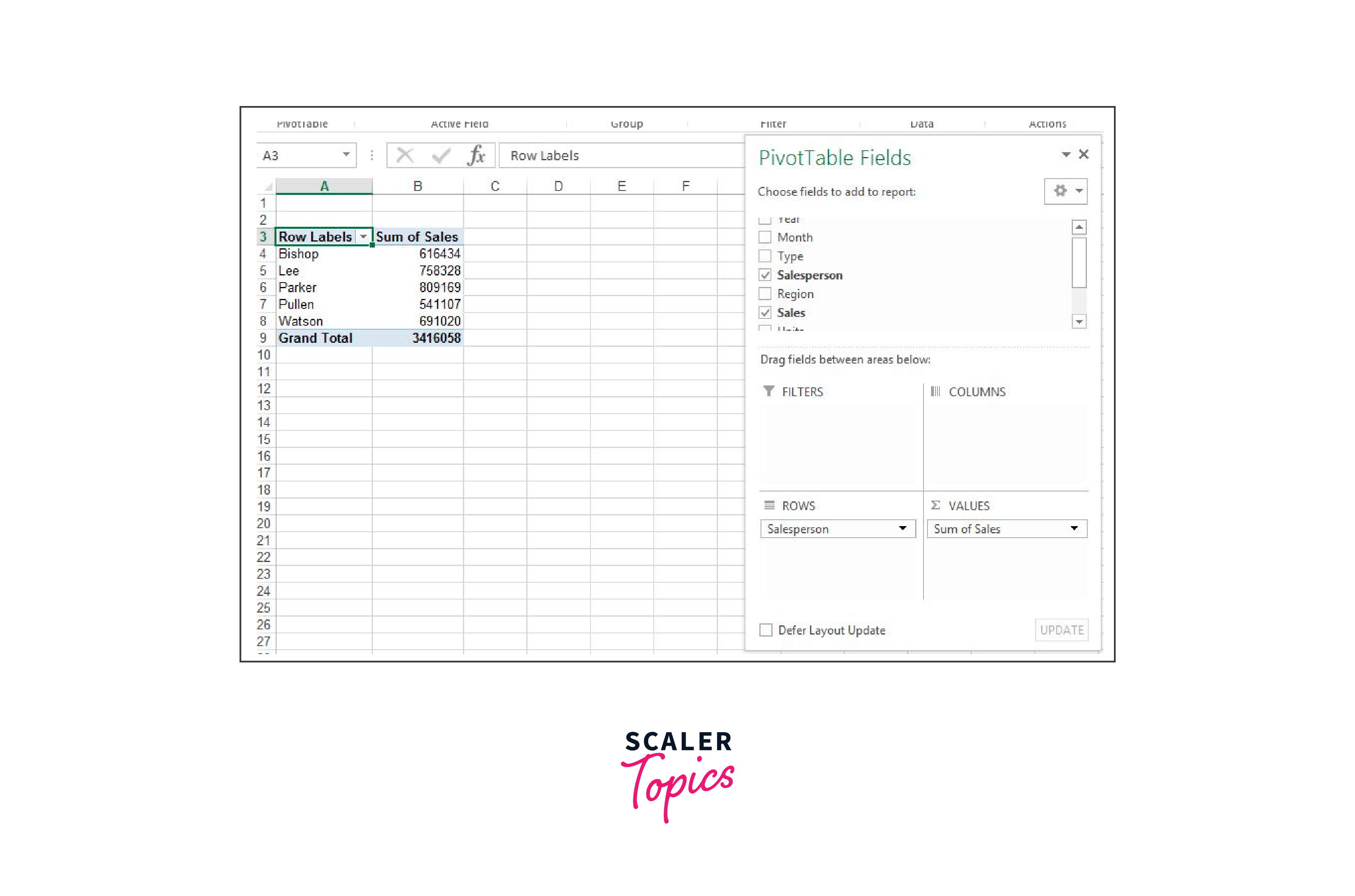
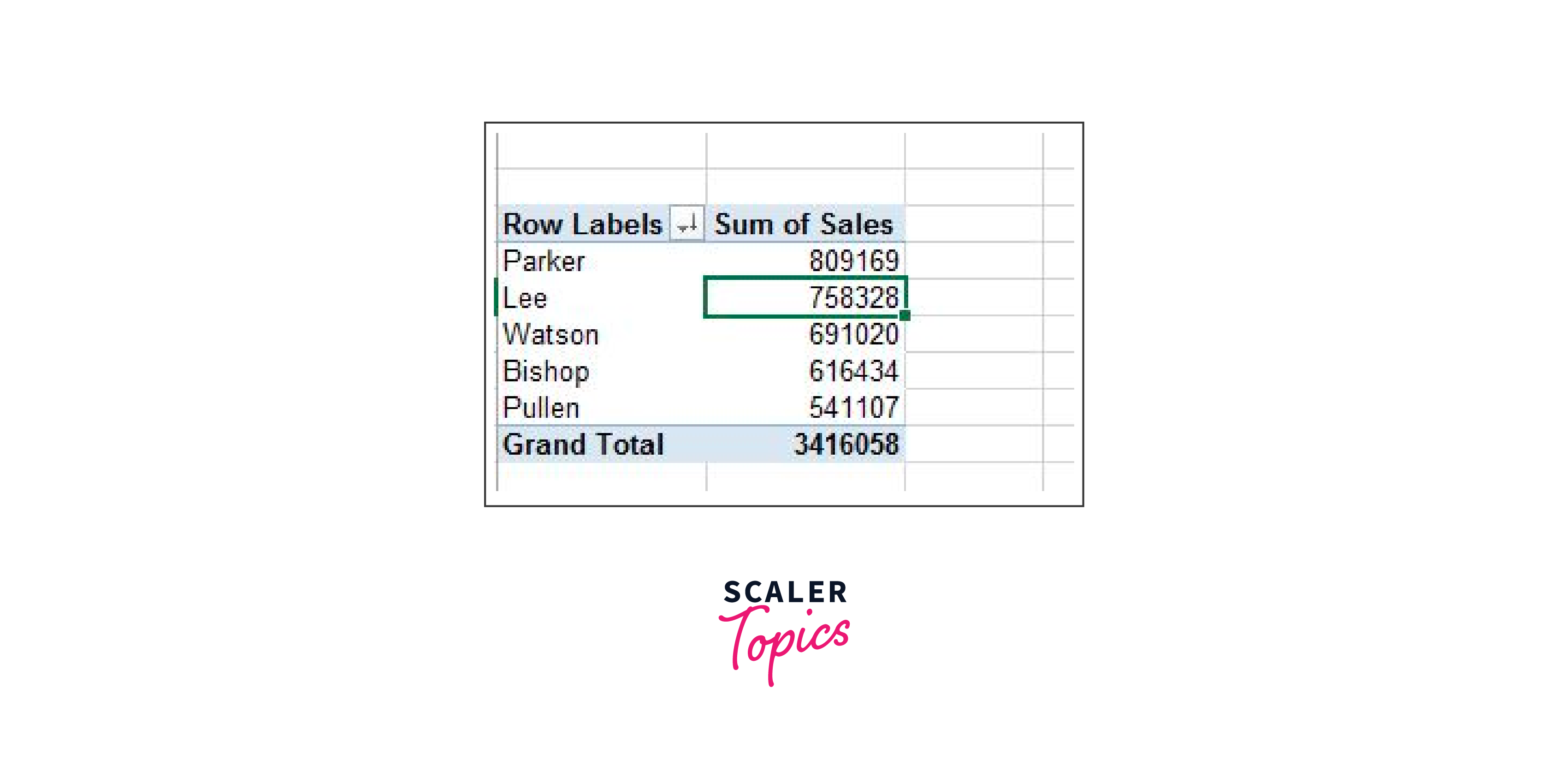
Drag the following fields to the following locations to obtain each salesperson's total sales.

Field salesperson to the Rows area. Values are to the Sales field.

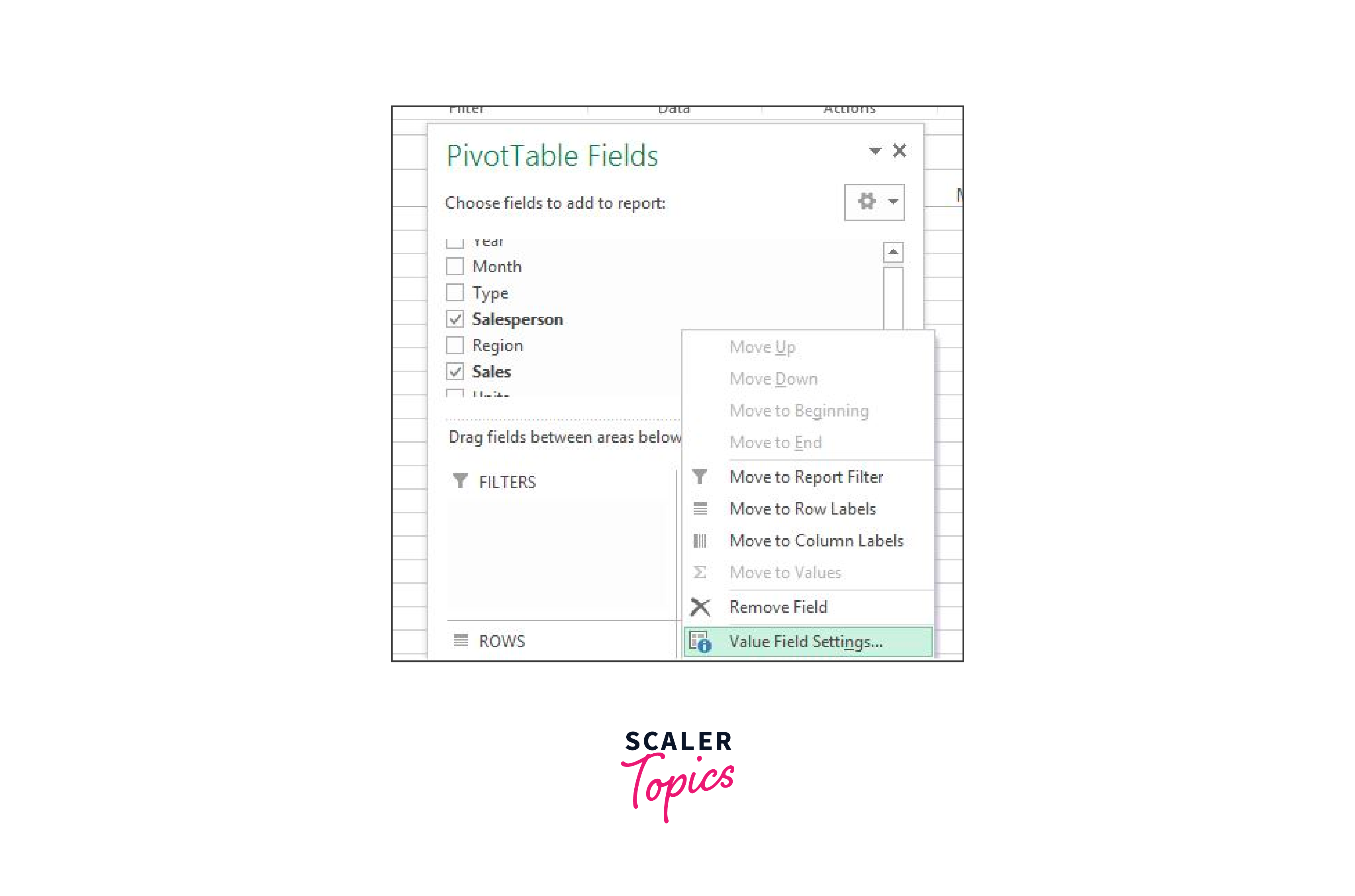
Value Field Settings

Excel, by default, displays the total of the values entered in the Values section. However, that can be modified in the Value Field Settings.

In the Values area, select the Sum of Sales.

Select the calculation type you want to use.

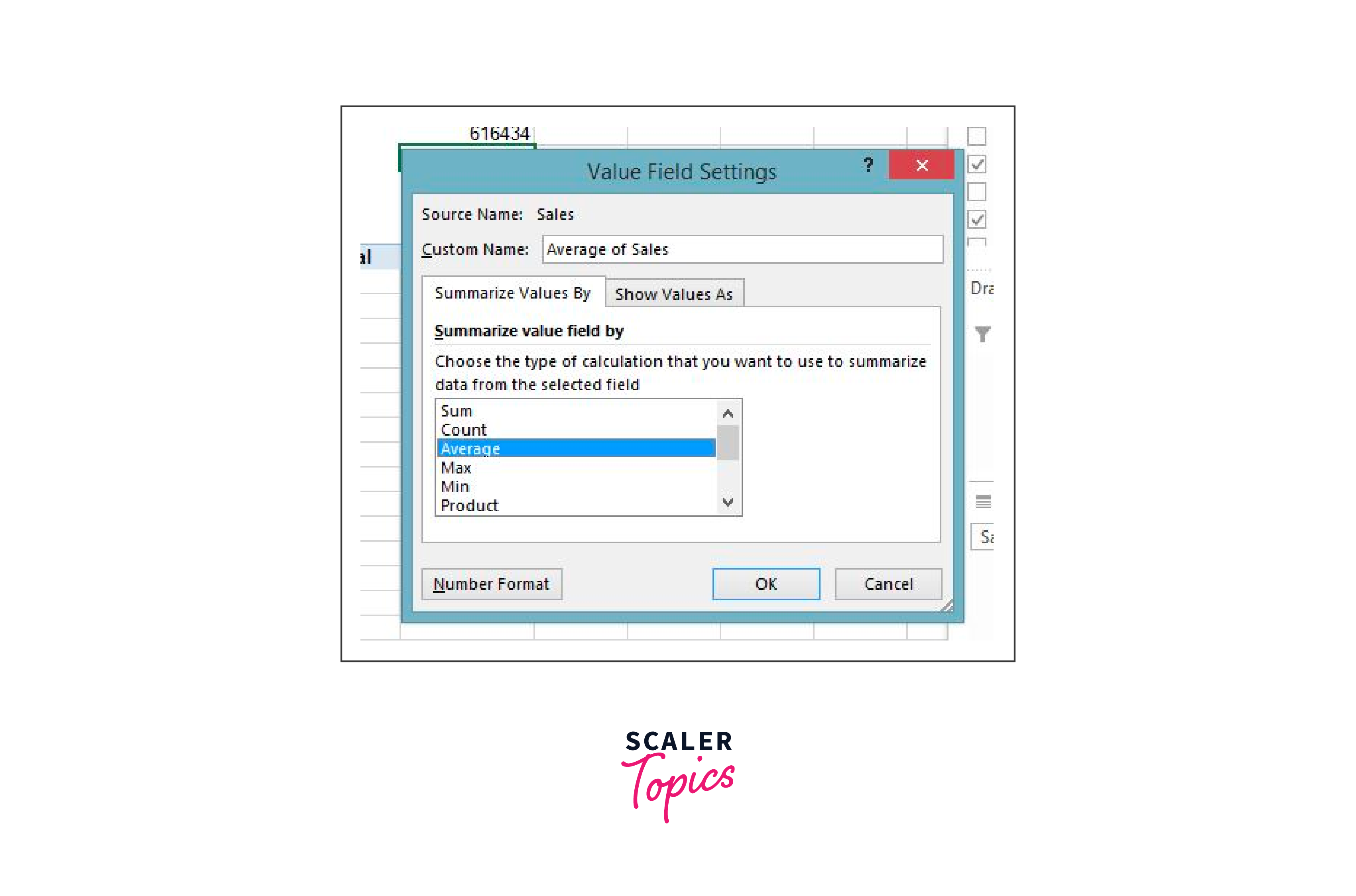
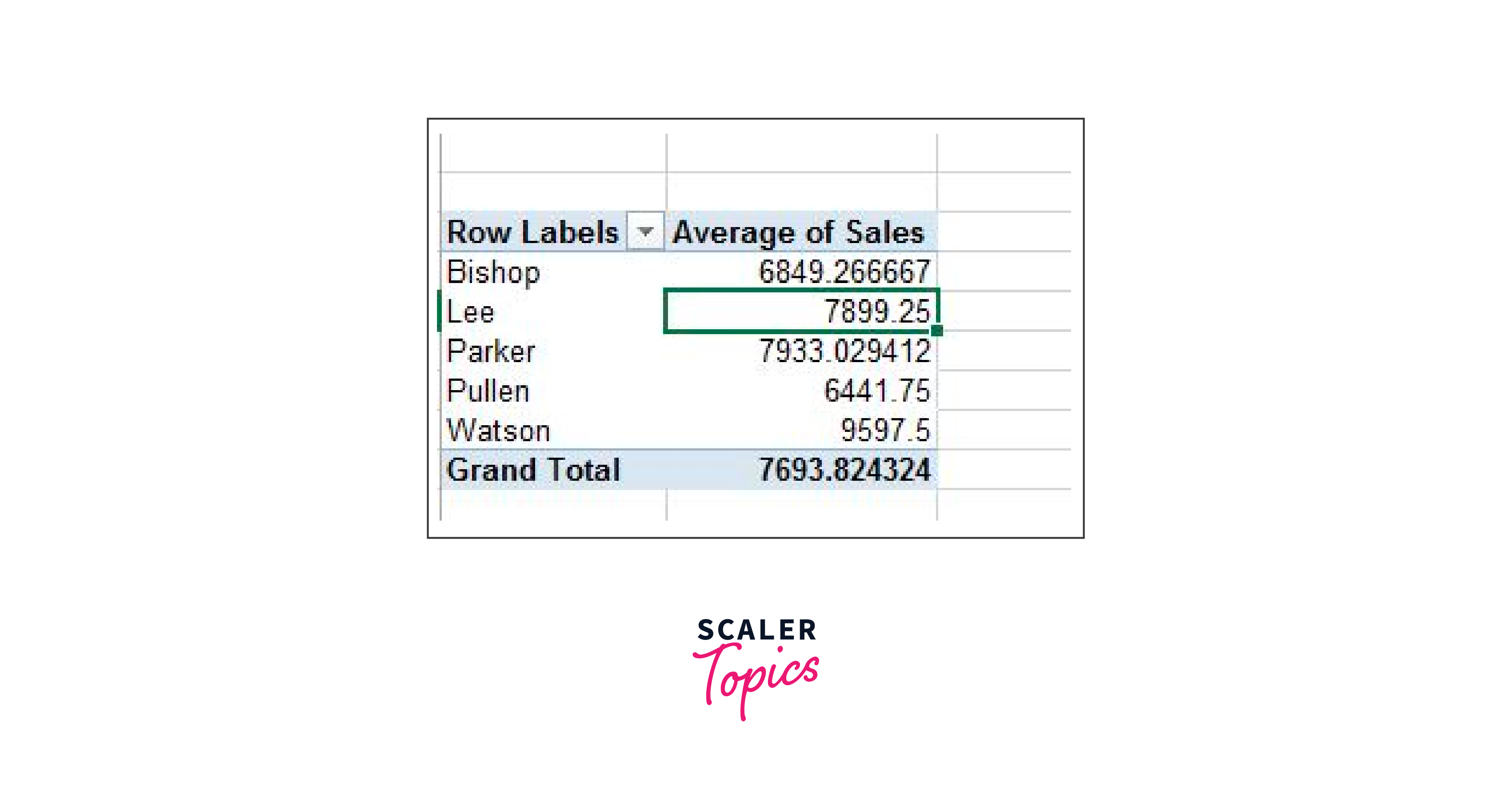
Click OK.

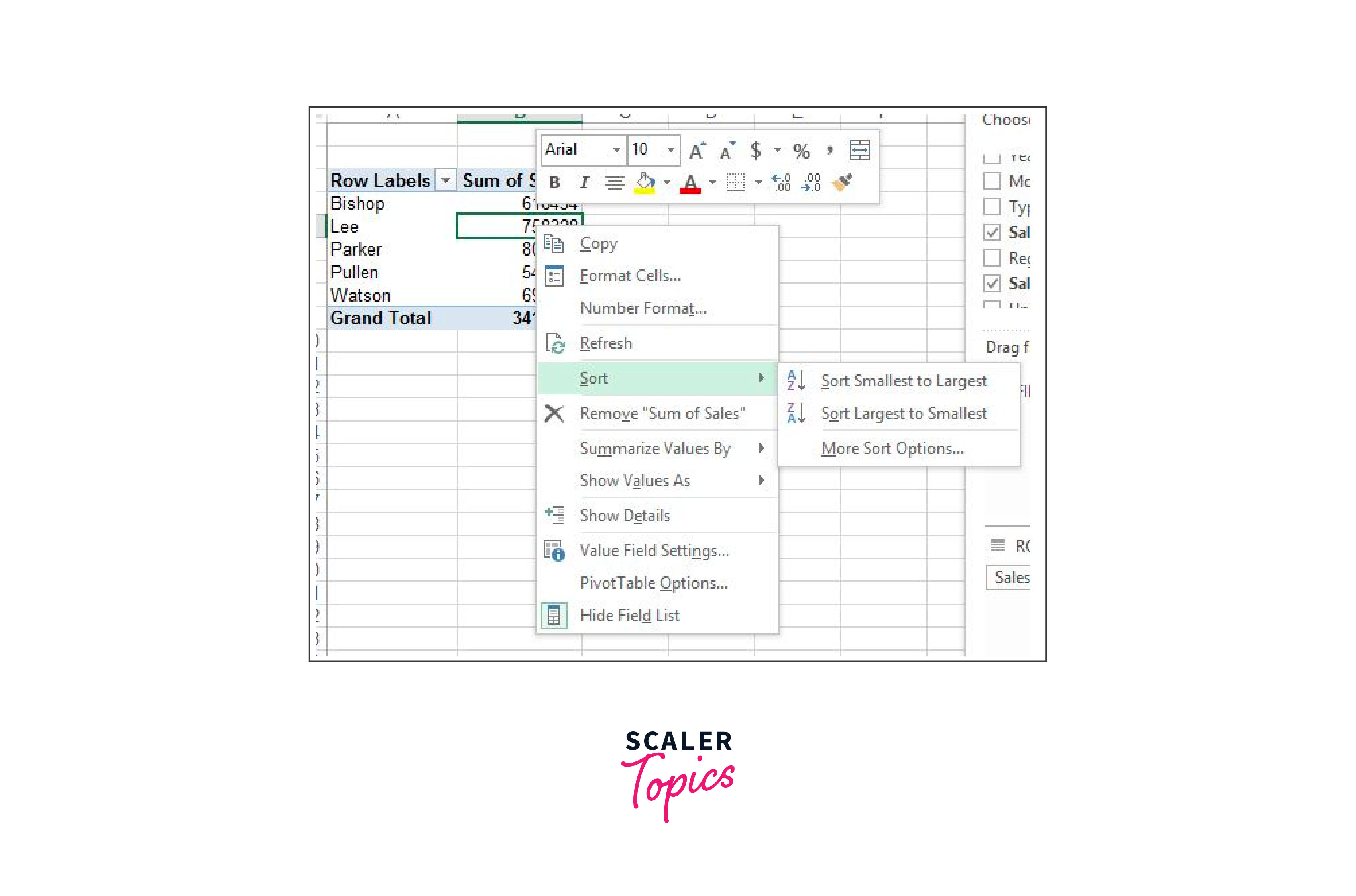
Sort

Click any sales value in the context menu and select Sort > Sort Largest to Smallest.

Result:

Filter

Filtering is the final piece of the puzzle that is sometimes left out when discussing pivot tables.

Simply removing some of the data rows (records) from the source table is filtering.

The generated Pivot Table only contains values that can pass filters.

Let's look at how we may give our pivot table a filter.

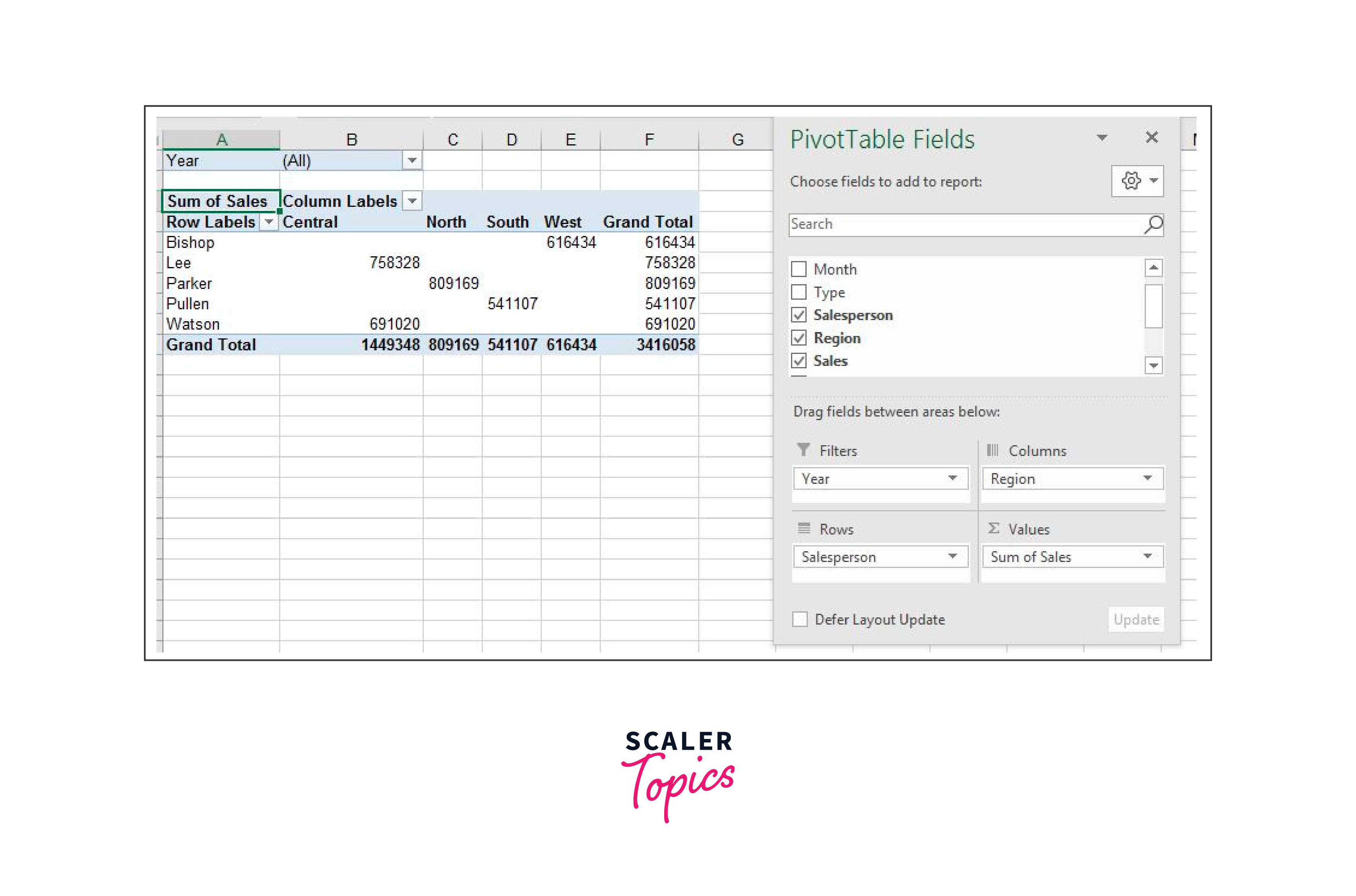
As you can see, it adds a filter to the worksheet's top.

Change Summary Calculation

By default, Excel counts or adds up the items to create a summary of your data. Follow the procedures below to alter the calculation type you want to use.

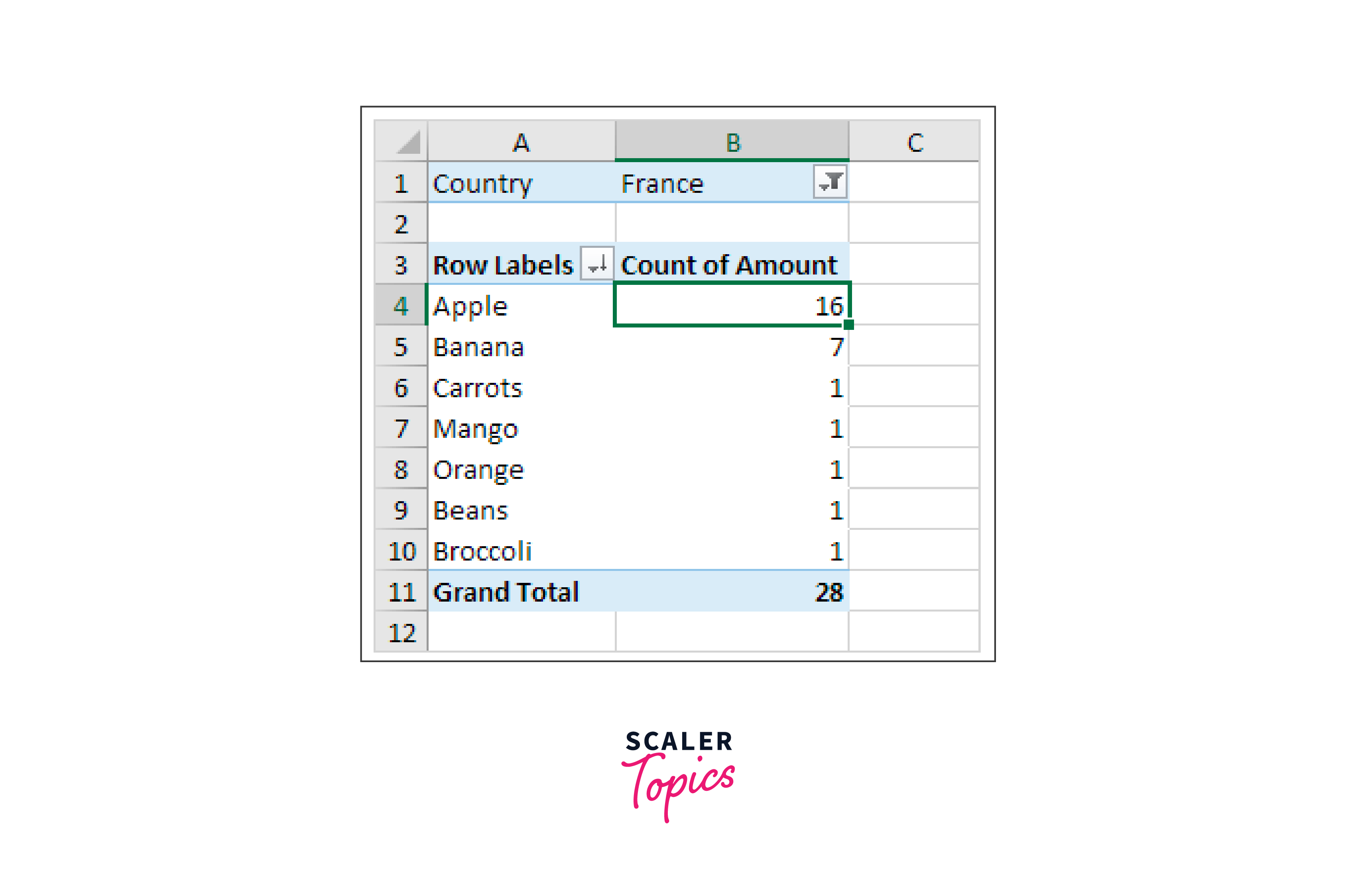
1. Select a cell from the Sum of Amount column by clicking it.

2. Select Value Field Settings with the right mouse click.

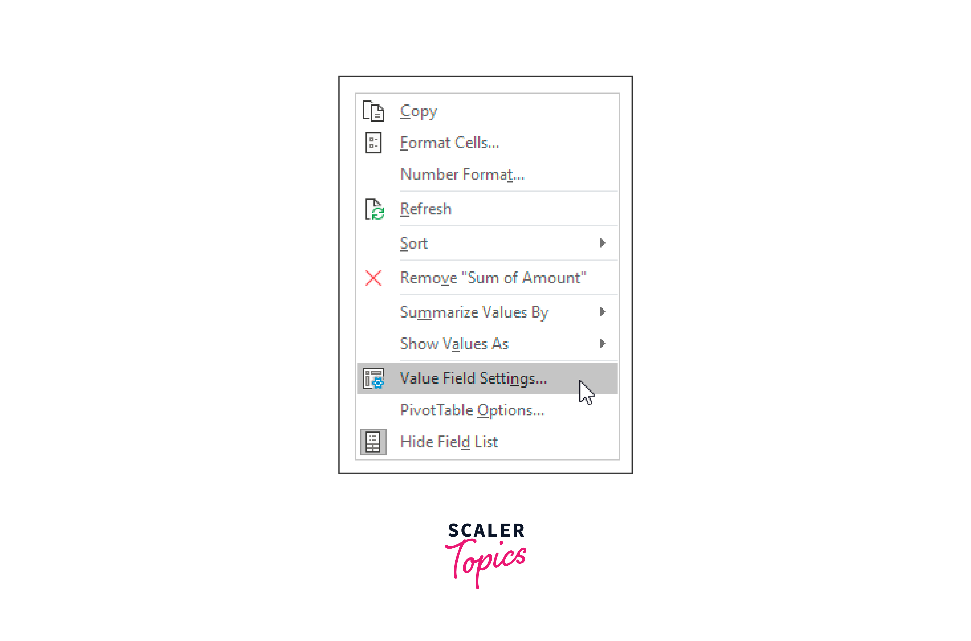
3. Decide on the calculation type you want to use. For instance, select Count.

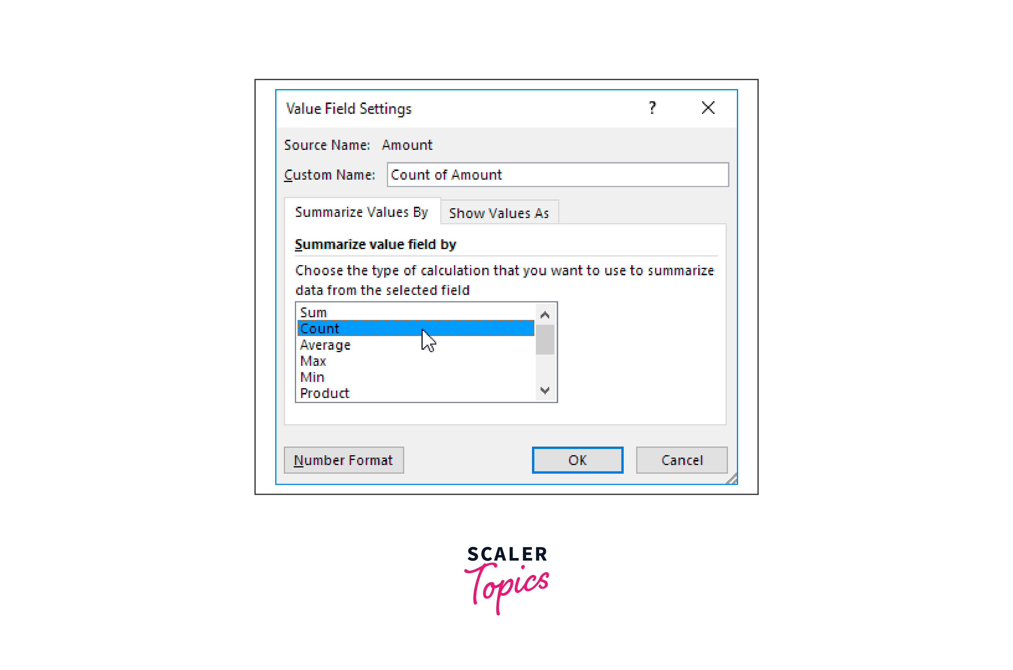
4. Click OK.

Result. 'Apple' orders comprised 16 of the 28 orders sent to France.

Two-dimensional Pivot Table

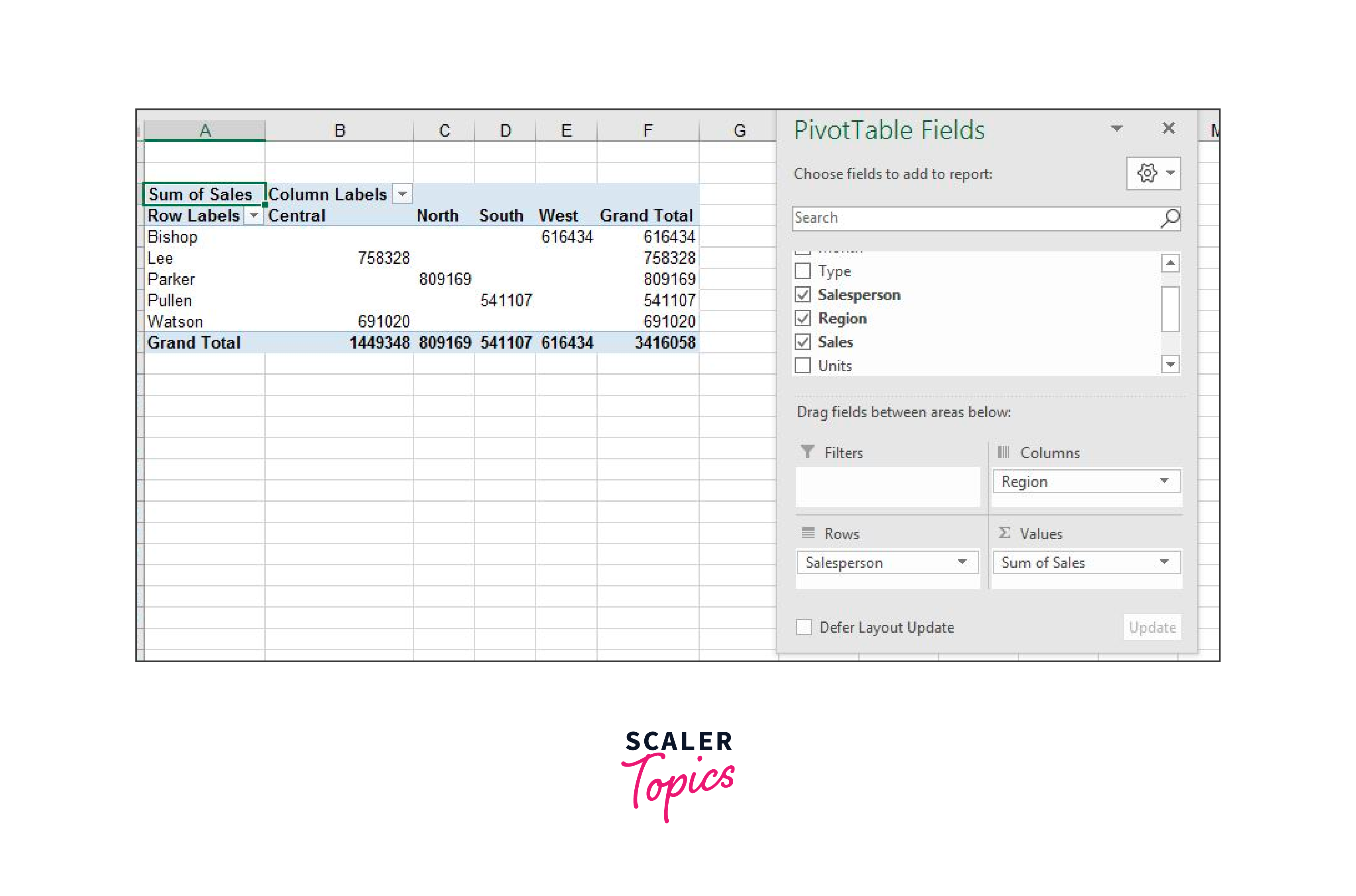
A pivot table in excel can be set up in different two-dimensional configurations. Drag the following fields to the various spaces.

An area salesperson for Rows.

The area from region to columns.

Sales directed at Values.

Refresh Pivot Table

You might be surprised that Excel does not immediately refresh even if a Pivot Table report is linked to your source data. Any data changes can be obtained manually, or they can be obtained automatically when you access the spreadsheet.

Refresh the Pivot Table data manually.

Click anywhere on your table.

Click the Refresh button or press ALT+F5 in the Data group of the Analyse tab (the Options tab in previous iterations).

The table can also be selected by right-clicking it and selecting Refresh from the context menu.

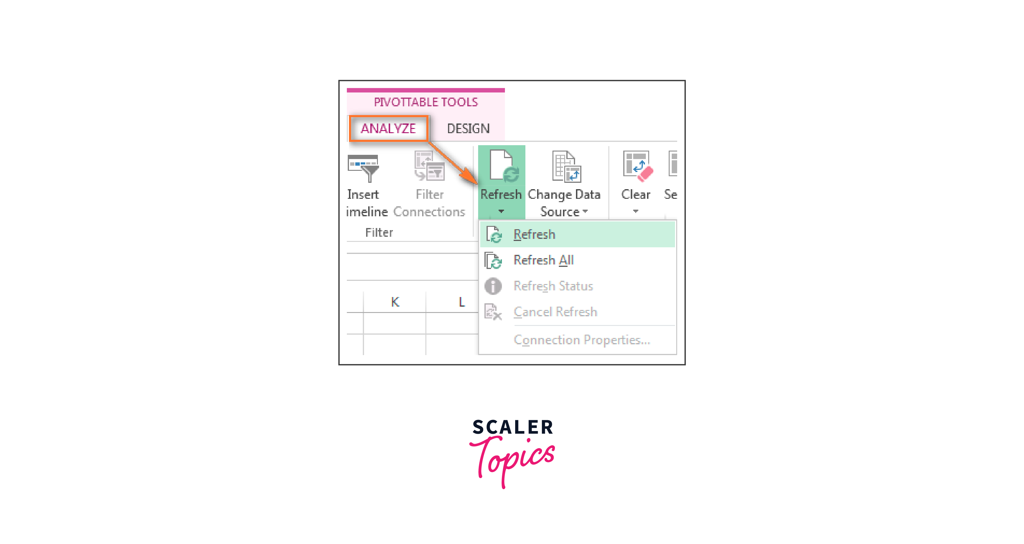
Click the arrow next to the Refresh button to open the menu, then select Refresh All to update every Pivot Table in your workbook.

Ensure the "Autofit column width on update" and "Preserve cell formatting on update" settings are checked if your Pivot Table's format changes after refreshing. To verify this, click the Analyse (Options) tab > PivotTable group > Options button. These checkboxes are located on the Layout & Format tab of the PivotTable Options dialogue box.

You can check the status after starting a refresh or stop it if you've changed your mind. Click the arrow next to the Refresh button and select Refresh Status or Cancel Refresh.

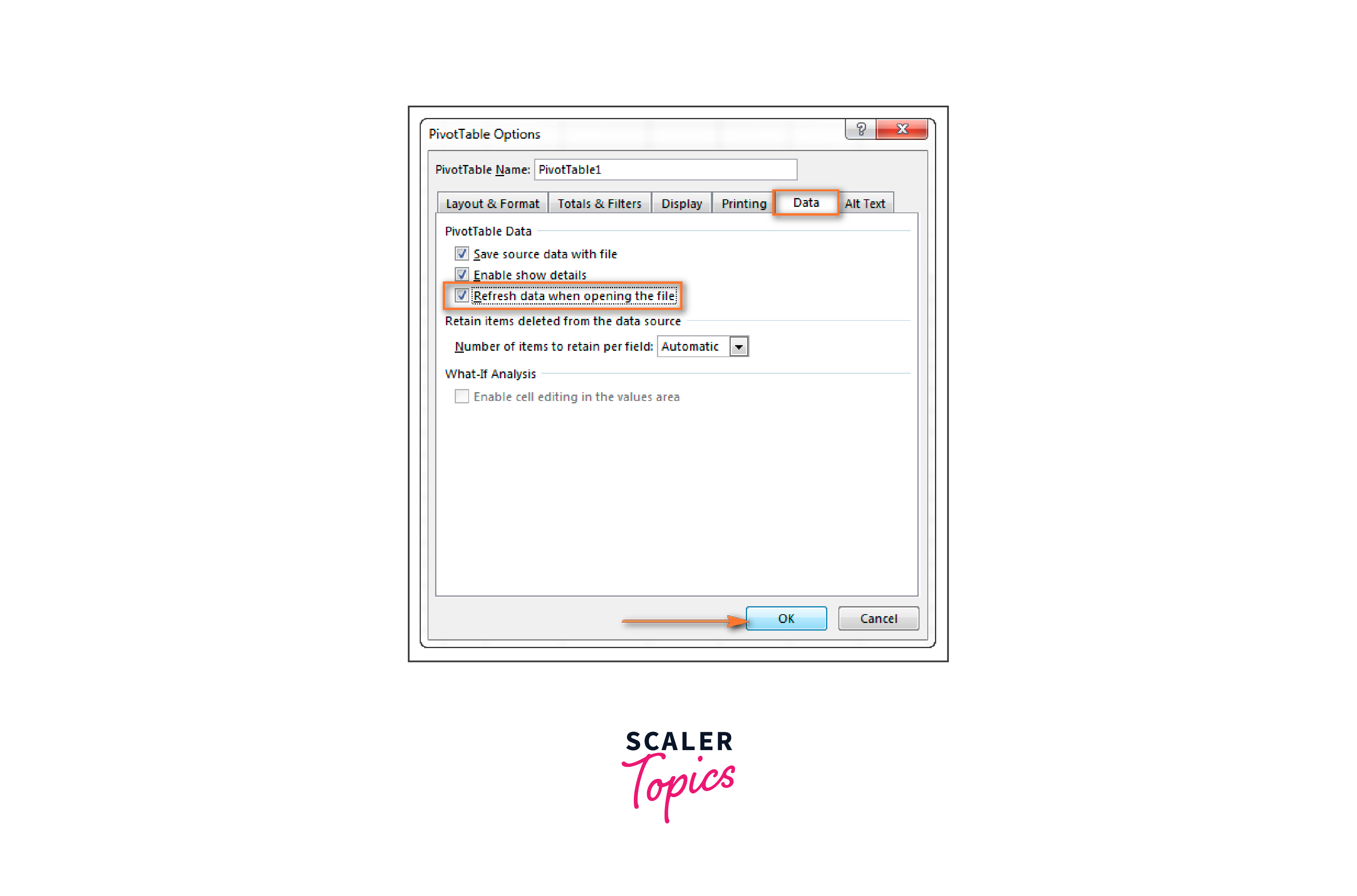
Refreshing a Pivot Table automatically when opening the workbook Click Options > Options under the PivotTable group on the Analyse / Options tab.

Select the Refresh data when opening the file check box on the Data tab of the PivotTable Options dialogue box.

Move the Pivot Table to a New Location

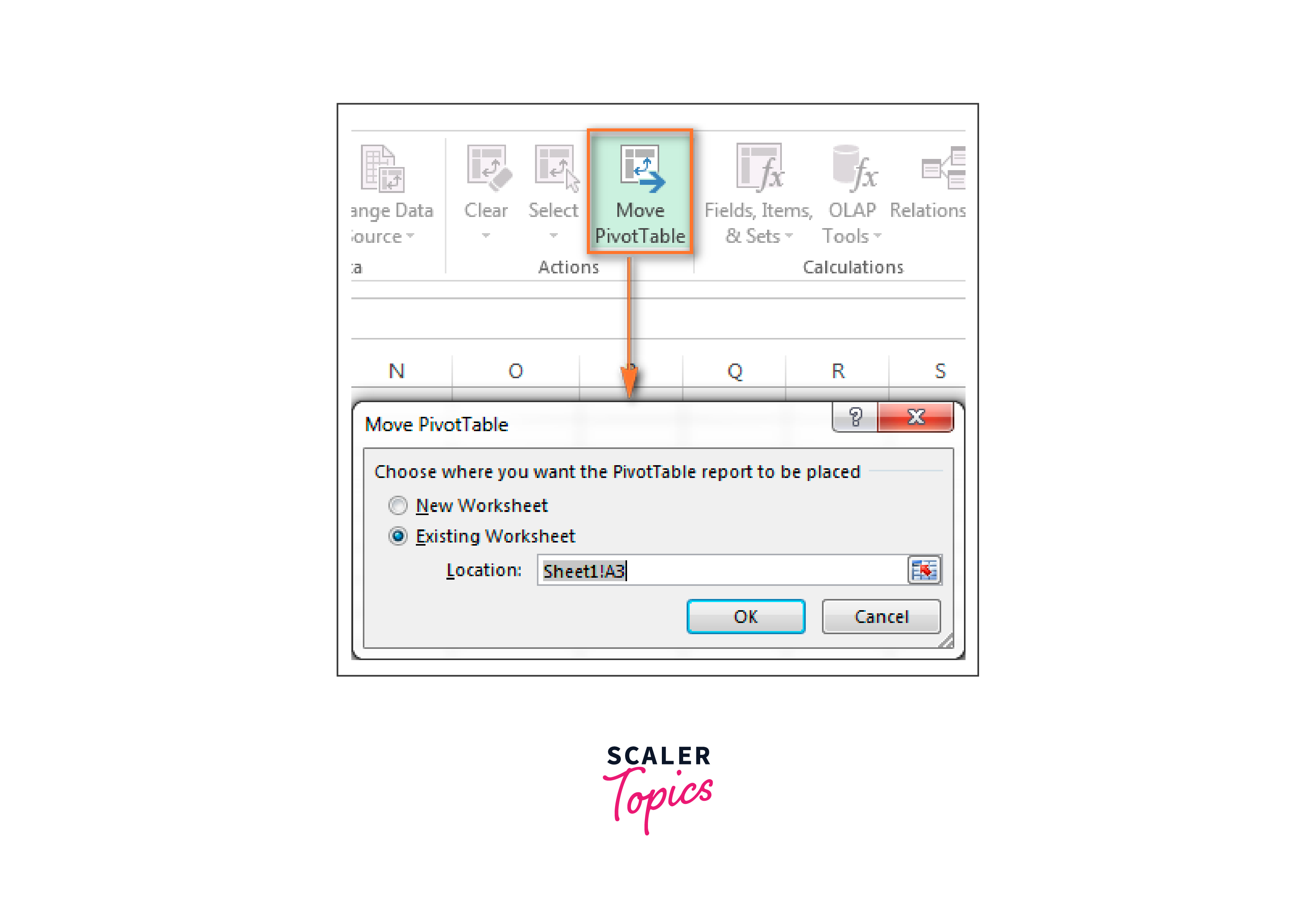
Click the move PivotTable button in the Actions group on the Analyse tab (the Options tab in Excel 2010 and prior) to relocate your pivot table to a different workbook, worksheet, or section of the current sheet. Click OK after choosing a different location.

Delete Pivot Table

There are several ways to delete a summary report you no longer require.

• Simply delete that sheet if your table is on a different worksheet.
• Select the entire Pivot Table with the mouse and press the Delete key if your table is on a sheet with other data.
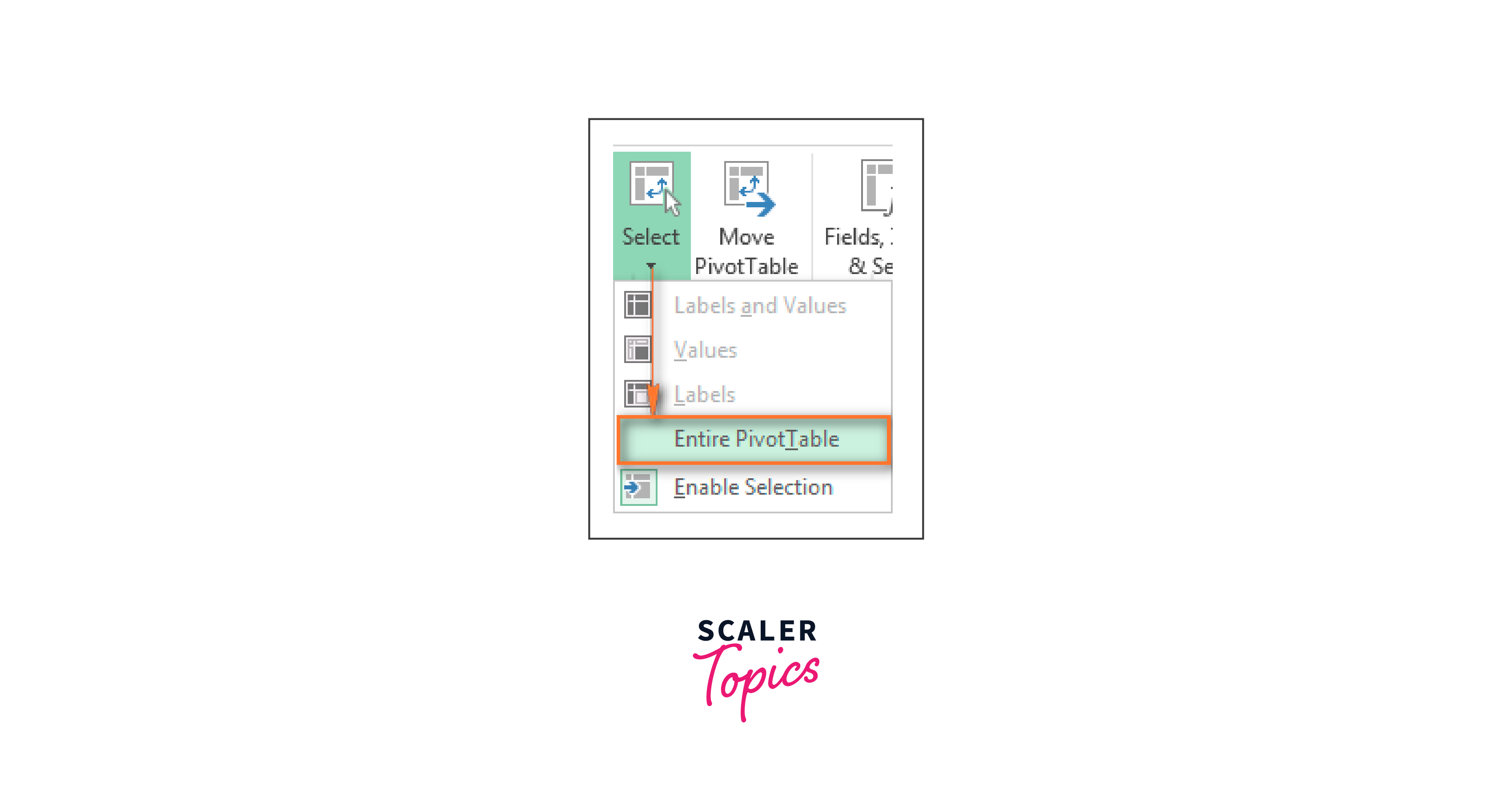
• Click anywhere in the pivot table you want to delete, choose Entire PivotTable from the Actions group on the Analyse tab (the Options tab in Excel 2010 and prior), and then press the Delete key.

It should be noted that deleting the pivot table would convert all associated PivotTable charts into standard charts that cannot be changed or twisted.