Poisson Regression in R
Overview
Poisson regression in R is a statistical technique that plays a pivotal role in modeling count data across diverse fields. In this article, we delve into the intricacies of this method, exploring its mathematical underpinnings, applications, and implementation in R. Poisson regression is designed to predict event counts within a fixed interval, making it invaluable for scenarios like forecasting customer arrivals, accidents, or email volumes. Unlike the normal distribution, it caters to discrete data and effectively handles overdispersion. Poisson regression is a subset of Generalized Linear Models (GLMs), offering a unified approach to regression analysis. With R's robust libraries and functions, fitting Poisson regression models to your data becomes accessible and efficient.
Introduction to Poisson Regression
Poisson regression in R is a statistical method that proves invaluable when dealing with count data analysis. Whether you're predicting customer arrivals at a store, accidents at an intersection, or the number of emails received, Poisson regression offers a robust framework for modeling these discrete events within fixed intervals.
At its core, Poisson regression extends the concept of the Poisson distribution to regression analysis. It allows us to predict event counts while considering multiple predictor variables. The heart of the model lies in its ability to express the expected event count as a linear combination of these predictors. In R, this technique is easily implemented, making it a vital tool in a data analyst's arsenal.
Mathematical Formuala for Poisson Regression
To understand Poisson regression in R, it's crucial to grasp the underlying mathematical formula that governs this statistical technique. At its core, Poisson regression is rooted in the Poisson distribution, a probability distribution commonly used for modeling count data.
The Poisson distribution is defined by a single parameter, λ (lambda), which represents the average event rate. The probability mass function of the Poisson distribution is given by:
λ (lambda) in the Poisson distribution represents the practical average rate of events occurring within a specified timeframe or space. For example, if we are tracking customer arrivals at a store, λ signifies the average number of customers expected to arrive during that time period. It serves as a crucial parameter for understanding and modeling event occurrences in real-world situations.
Here's a breakdown of the components in this formula:
- P(X = x):
This represents the probability that the random variable X takes on the value x, which is a specific count of events. - e:
This is the base of the natural logarithm, approximately equal to 2.71828. - λ:
Lambda, the parameter of the Poisson distribution, denotes the average rate at which events occur. - x:
The count of events we want to calculate the probability for. - x!:
The factorial of x, which is the product of all positive integers from 1 to x.
The Poisson regression model builds upon this foundation. It allows us to predict event counts while considering multiple predictor variables. The central idea is that the logarithm of the expected event count (λ) is a linear combination of these predictors.
The general form of the Poisson regression model can be expressed as:
Here, β₀, β₁, β₂, ..., βₖ are the model coefficients, and X₁, X₂, ..., Xₖ are the predictor variables.
What are Poisson Regression Models?
Poisson regression models in R are statistical tools used to predict counts of events or occurrences. These models are particularly useful when you're dealing with data that involves counting discrete events within a fixed interval, like the number of customers arriving at a store, the number of accidents at an intersection, or the number of website clicks in an hour. Let's dive deeper into what makes Poisson regression models special:
- Mathematical Foundation:
Poisson regression models are built upon the Poisson distribution, characterized by a single parameter, λ (lambda), representing the average event rate. The probability mass function of the Poisson distribution is used as the basis for these models:
In this formula, X represents the count of events, x is a specific count value, e is the base of the natural logarithm, and λ is the average event rate.
- Predictive Power:
The primary objective of Poisson regression models is to predict the count of events based on one or more predictor variables. For instance, in a retail setting, you might want to predict the number of customers visiting a store based on factors like day of the week, advertising expenditure, and location. - Linear Relationship:
Poisson regression models assume that the log of the expected event count (λ) is a linear combination of the predictor variables. The general form of the Poisson regression model can be written as:
Here, β₀, β₁, β₂, ..., βₖ are the model coefficients, and X₁, X₂, ..., Xₖ are the predictor variables.
- Flexibility:
Poisson regression models can handle both categorical and continuous predictor variables, making them versatile for a wide range of applications in fields such as epidemiology, economics, and social sciences.
Example in R:
Let's create a simple example using dummy data to demonstrate Poisson regression in R. In this example, we'll predict the number of customer purchases based on two predictor variables: advertising expenditure and the day of the week.
Output:
In this code, we've created a dataset with 100 rows. advertising_expenditure represents the amount spent on advertising, day_of_week represents the day of the week (1-7, where 1 is Sunday), and purchases represents the number of customer purchases.
This code uses the glm function to fit a Poisson regression model. The purchases variable is the response variable, and advertising_expenditure and day_of_week are the predictor variables. We specify the family argument as poisson to indicate that we are fitting a Poisson regression model.
How Does Poisson Distribution Differ From Normal Distribution?
Here's a concise table highlighting the key differences between the Poisson distribution and the Normal distribution:
| Characteristic | Poisson Distribution | Normal Distribution |
|---|---|---|
| Type of Distribution | Discrete | Continuous |
| Purpose | Models event counts | Models continuous data |
| Parameter | λ (lambda) - Average event rate | μ (mu) - Mean and σ (sigma) - Standard Deviation |
| Probability Mass Function (PMF) | ||
| Range of Values | Non-negative integers | All real numbers |
| Mean and Variance | Mean = λ, Variance = λ | Mean = μ, Variance = σ² |
| Shape | Right-skewed (as λ increases) | Bell-shaped, symmetric |
Poisson Regression Models and GLMs
Poisson regression, as we've discussed earlier, excels at predicting event counts based on predictor variables. GLMs, on the other hand, provide a unified framework that extends beyond linear regression. Let's explore how these two concepts come together to enhance our understanding of data.
Poisson Regression Models
Poisson regression models, as the name suggests, are tailored to work with count data, making them an invaluable tool in various fields. They are the go-to choice when you need to predict event counts, and they make it possible to include multiple predictor variables in your analysis. The core mathematical formula of Poisson regression is:
Where β_0, β_1, β_2, ..., β_k are coefficients, and X_1, X_2, ..., X_k are predictor variables.
Generalized Linear Models (GLMs)
GLMs are a versatile class of statistical models that encompass various regression techniques. They offer a unified approach to modeling, allowing us to handle different types of response variables and error distributions. Poisson regression is one of the stars in the GLM galaxy, specifically designed for count data.
Here's how Poisson regression fits into the GLM framework:
- Link Function:
GLMs introduce a concept called the link function, which connects the linear predictor (the right side of the Poisson regression equation) to the expected value of the response variable. For Poisson regression, the default link function is the natural logarithm (log-link), as shown in the formula. - Family of Distributions:
GLMs allow you to choose a family of distributions that best suits your data. In the case of Poisson regression, you specify the family as "poisson" to indicate that you're working with count data.
Example in R
Let's consider a scenario where we want to predict the number of customer purchases based on advertising expenditure and day of the week, just like in the earlier example. This time, we'll use the glm function in R to fit a Poisson regression model within the GLM framework:
In this example, the family argument is set to poisson to specify that we're using Poisson regression within the GLM framework.
Modelling
We're about to dive into modeling Poisson Regression using R, focusing on how frequently yarn breaks during weaving. We'll work with the warpbreaks dataset, which is included in the datasets package in R. First, ensure you have the datasets package installed.
The datasets package contains a wide array of datasets, and for this example, we'll specifically use the warpbreaks data.
What is in Our Data?
The warpbreaks dataset explores the number of warp breaks that occurred for different types of looms, per loom, and per fixed length of yarn. It consists of three columns:
- breaks:
This is a numerical variable representing the count of breaks. - wool:
This variable is categorical and indicates the type of wool used, which can be either A or B. - tension:
Similarly, this categorical variable denotes the level of tension, which can take on values of L, M, or H.
There are measurements for 9 looms of each of the six types of warp, resulting in a total of 54 entries in the dataset.
Now, let's examine the structure of the data using ls.str(warpbreaks):
Output:
Modeling the Poisson Regression
We are interested in predicting the number of warp breaks (response variable) based on the predictor variables wool and tension. To achieve this, we'll use a Poisson regression model.
Output:
Interpreting the Poisson Model
Interpreting the results from our Poisson regression model, we can analyze the coefficient estimates:
- exp(α):
This represents how the mean μ changes when the predictor variable X is set to 0. - exp(β):
This signifies that for every one-unit increase in X, the predictor variable has a multiplicative impact of exp(β) on the mean value of Y (μ).
Consider the scenario where β takes on different values in Poisson regression. When β equals 0, exp(β) equals 1, implying that the expected count aligns with exp(α), signifying no significant relationship between the variables Y and X. However, when β is greater than 0, exp(β) exceeds 1, signifying that for each unit increase in X, the expected count becomes exp(β) times larger than when X equals 0. Conversely, if β is less than 0, exp(β) is less than 1, suggesting that the expected count is exp(β) times smaller than when X is set to 0. These interpretations illuminate the impact of different β values on the expected outcome in Poisson regression.
Therefore, we can utilise a quasi-poisson model to have a standard error that is more accurate:
Output:
Comparing Models
We can compare different models using the jtools package. First, install it if not already installed (install.packages("jtools")), and then load the library.
Now, you can compare models and visualize their coefficients and interactions using functions like plot_summs() and cat_plot() from the jtools package. These visualizations help you understand the model and its effects better.
- plot_summs():
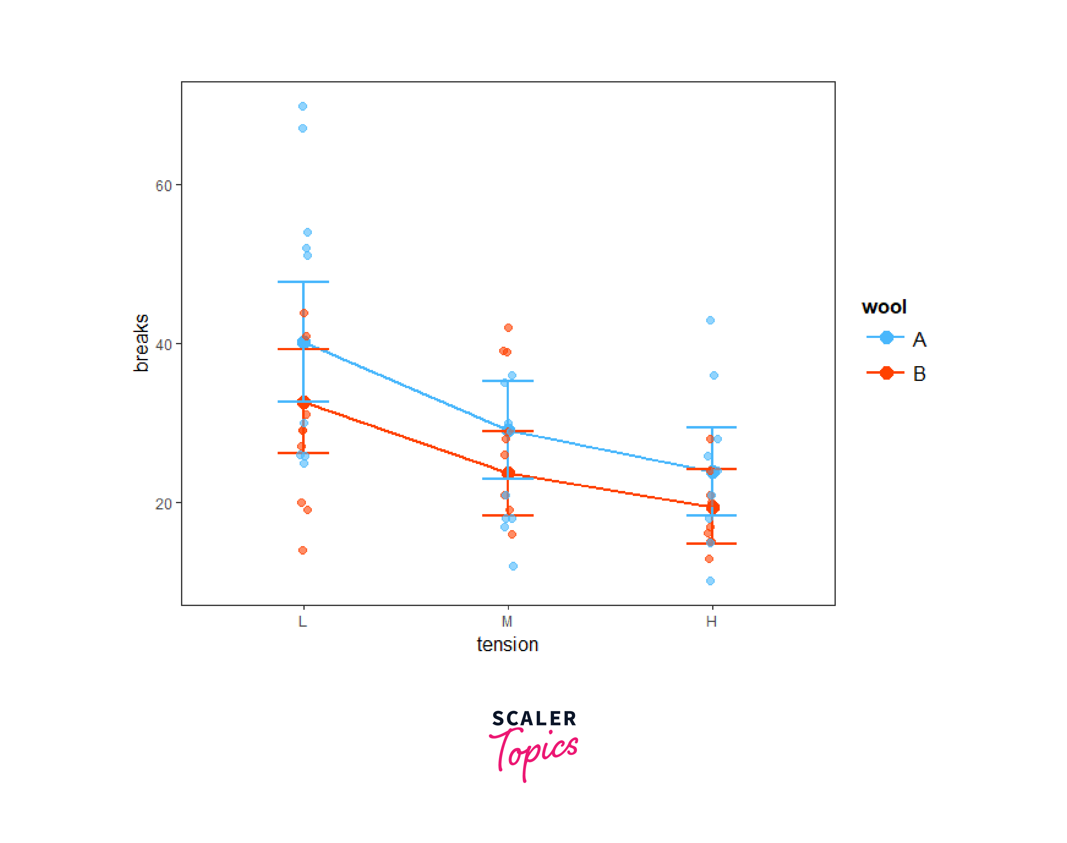
This visualization summarizes the coefficients of regression models, making it easier to interpret their effects. It typically displays coefficient values, their standard errors, and often their exponentiated values. It helps you understand the significance and direction of each predictor variable's impact on the response variable. - cat_plot():
This function is particularly useful when dealing with categorical variables. It visualizes how different categories or levels of predictors interact and affect the response variable. By examining these plots, you can gain insights into how combinations of categorical variables influence the outcome.
Predicting From the Model
To make predictions from your Poisson regression model for new data, you can use the predict() function. Provide the model, new data, and specify the type of prediction you want.
In this example, we predict that there will be roughly 24 breaks with wool type B and tension level M.
Visualizing Findings Using jtools
Visualization is essential for sharing your analysis effectively. The jtools package provides tools for summarizing and visualizing regression models. For instance, you can use plot_summs() and cat_plot() to visualize the summary of your Poisson regression model and explore interactions among variables.
Here's how to use plot_summs():
And to visualize interactions between categorical variables using cat_plot():
Conclusion
- Poisson regression in R is a powerful tool for modelling count data, allowing you to predict event counts based on predictor variables.
- Poisson regression seamlessly integrates into the broader framework of Generalized Linear Models (GLMs), providing flexibility in modelling different types of data and responses.
- Understanding the exponentiated coefficients in Poisson regression helps us grasp the multiplicative effects of predictor variables on the response variable, making it a valuable tool for analyzing count data.
- Utilizing packages like jtools enables us to visualize and communicate our findings effectively, facilitating a deeper understanding of the model's effects and interactions.
- Poisson regression in R has applications across various fields, from predicting customer purchases to analyzing industrial process data, making it an indispensable statistical tool for count data analysis.
- Embracing the intricacies of Poisson regression and its applications is an ongoing journey in the realm of statistical analysis. Continuous learning and exploration in this field can empower you to harness the full potential of Poisson regression for tackling complex real-world challenges.