Cardinality Of Relationship In Power BI
Overview
In Power BI, one of the fundamental aspects of data modeling is defining relationships between tables. The cardinality of these relationships plays a crucial role in determining how data is combined and analyzed in reports and visualizations. Understanding the cardinality options, such as "One-to-One," "One-to-Many," and "Many-to-Many," is essential for creating efficient and accurate data models. In this article, we will explore the concept of cardinality in Power BI, its significance, and practical examples of how to set up and use different relationship types to optimize data analysis and reporting.
What are Power BI Model Relationships?
Power BI Model Relationships play a pivotal role in connecting data tables within a model and enable the seamless flow of filters from one table's column to another. These relationships allow data aggregation and analysis across multiple tables based on defined cardinality settings.
Filters are propagated along relationship paths without any random variation, ensuring consistent results. However, specific DAX functions in model calculations can override or modify filter context for relationships.
Let's consider an example to understand better how Power BI model relationships work. In this scenario, we have a model comprising four tables - Category, Product, Year, and Sales. All interconnected through one-to-many relationships. The Category table is linked to the Product table, which in turn is linked to the Sales table. The Sales table is also linked to the Year table. Every relationship is one-to-many, as shown in the below figure. For instance, a query requests the total sales quantity for sales orders in the category "Cat-A" during the year "CY2018."
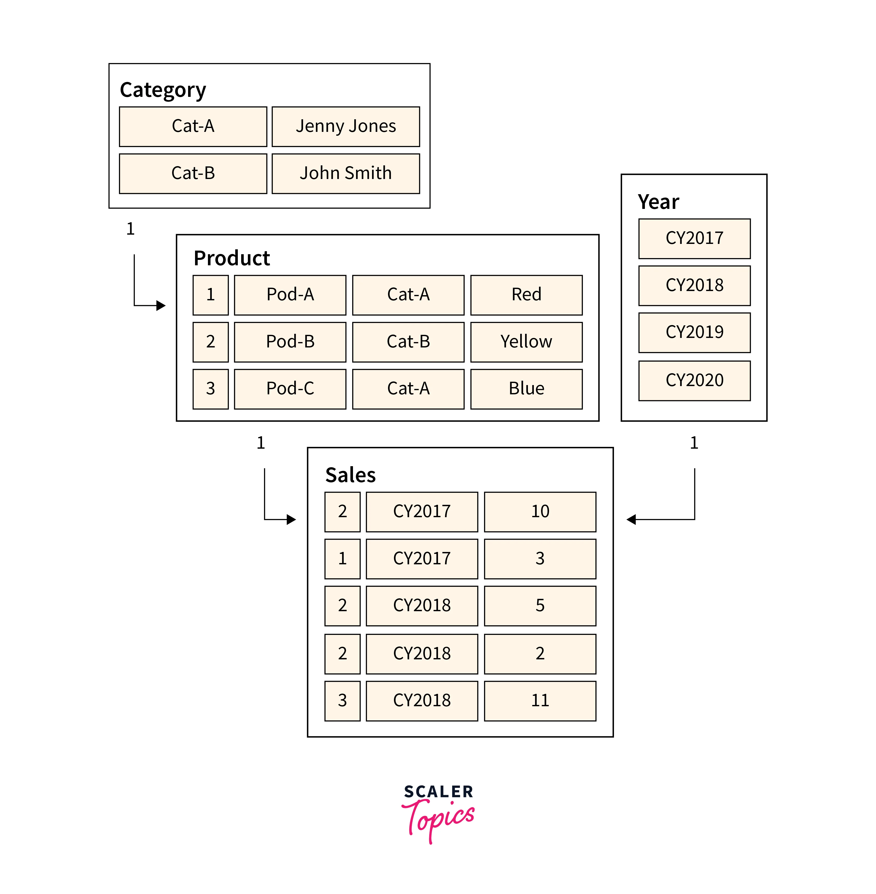
The Category and Year tables have filters applied, which propagate to the Product and Sales tables, respectively. The filters narrow down the dataset, isolating two products belonging to the category "Cat-A." The propagated filters on the Sales table then result in only two sales rows for these products, with a total of units. Simultaneously, the Year table's filter affects the Sales table, leaving only one sales row for products in the category "Cat-A" ordered in the year "CY2018," with a quantity value of 11 units. It's essential to understand that applying multiple filters always functions as an AND operation, requiring all conditions to be true.
This example demonstrates the significance of Power BI Model Relationships in guiding data flow and shaping the filter context, ultimately facilitating accurate and efficient data analysis for meaningful insights.
Power BI Model Relationships - Relationship Purpose
Apply Star Schema Design Principles
To build an effective model comprising dimensions and fact tables, it is highly recommended to adopt the star schema design principles. This approach in Power BI involves configuring rules that filter dimension tables, enabling Power BI model relationships to propagate these filters to fact tables seamlessly.
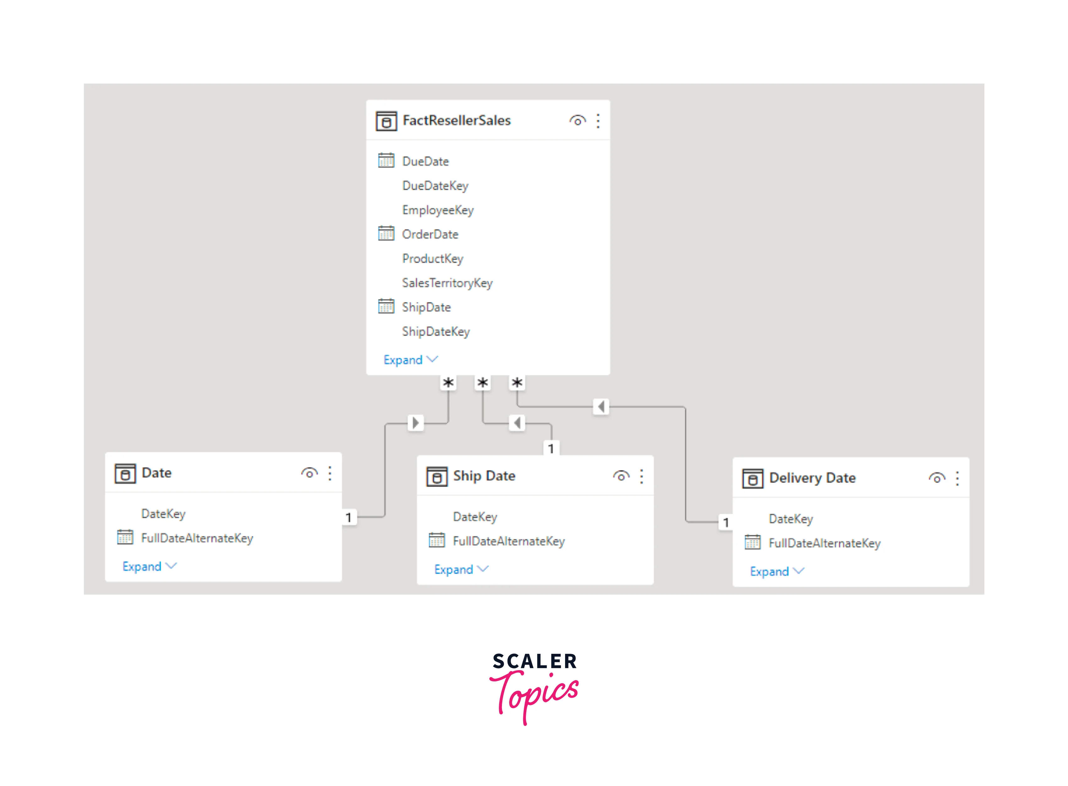
The model, shown in the below figure, illustrates the implementation of the star schema design. It consists of three main tables - Date, Ship Date, and Delivery Date, each establishing a single and active relationship with their corresponding reseller Sales table columns. This design not only simplifies data navigation and analysis but also enhances query performance, making it easier to uncover valuable insights from complex datasets.
Disconnected Tables
In Power BI model design, encountering a model table without a connection to another model table is relatively uncommon. Such tables are referred to as "disconnected tables," and they serve a unique purpose within a valid model structure. Filters originating from a disconnected table are not intended to propagate to other model tables. Instead, a disconnected table functions as a recipient of "user input," often facilitated through slicer visuals, enabling model calculations to derive meaningful insights from the provided value.
Let's consider an example of a disconnected table containing a range of currency exchange rate values. Through user input, such as selecting a specific rate value via a slicer, a measure expression can utilize that value to convert sales values accordingly.
Power BI Model Relationships - Understanding Relationship Properties
In Power BI, model relationships establish vital connections between columns in different tables, enabling seamless data integration and analysis. However, it's essential to note that relationships between columns within the same table are not supported in Power BI. This distinction is often confused with the concept of creating a table self-referencing relational database, commonly used to represent parent-child relationships (e.g., "reports to" relationship for each employee record).
Data Types Of Columns
In Power BI, columns in tables can have various data types, each serving specific purposes for data representation and analysis. Choosing the appropriate data types for columns is crucial for accurate data processing, efficient memory usage, and optimal visualizations in Power BI. Understanding these data types empowers users to effectively model and analyze diverse datasets, creating meaningful and insightful reports and dashboards. Some commonly used data types in Power BI include -
- Text/String -
This data type stores alphanumeric characters, such as names, descriptions, or any textual information. - Date/Time -
Date and time data types are employed to record date and time-related information, facilitating date-based analysis and time-series visualizations. - Boolean -
The Boolean data type stores True or False values, which are useful for representing binary conditions or logical decisions. - Integer -
The integer data type is used for storing non-decimal numeric values, suitable for counting and indexing purposes. - Decimal Number -
Decimal data types are ideal for storing numbers with a specific level of precision, making them suitable for financial calculations.
Cardinality
Cardinality in Power BI is a fundamental concept that defines the relationship between tables in a data model. It determines how data is combined and aggregated across related tables, playing a pivotal role in shaping the behavior of data analysis and visualizations.
Cardinality in Power BI holds immense significance in data modeling and analysis. It defines the relationships between tables in a data model, influencing how data is connected and aggregated across the entire dataset. By establishing these relationships, Power BI can seamlessly integrate data from various sources, enabling users to create comprehensive reports and visualizations that draw insights from interconnected information. Cardinality in Power BI ensures data consistency and integrity, as it governs how data is related, preventing any inconsistencies or inaccuracies in the final results. Furthermore, setting the right cardinality in Power BI plays a key role in optimizing query performance, leading to faster data retrieval and analysis. Properly defined cardinality empowers users to interpret data patterns accurately, make data-driven decisions, and gain valuable insights, making it an essential aspect of successful data modeling and reporting in Power BI.
Below are the four cardinality choices along with their shorthand notations -
- One-to-many
- Many-to-one
- One-to-one
- Many-to-many
When establishing a relationship in Power BI Desktop, it automatically detects and assigns the cardinality type. Power BI Desktop performs a query on the model to identify columns containing unique values, enabling it to determine the appropriate cardinality for the relationship intelligently. Now, let’s explore each type of cardinality in Power BI in the subsequent sections.
One-to-Many (and Many-to-One) Cardinality
The one-to-many and many-to-one cardinality options share similar characteristics and are among the most frequently used cardinality types.
When setting up a one-to-many or many-to-one relationship, you simply select the option that aligns with the order in which you linked the columns. For instance, consider configuring a relationship between the "Product" table and the "Sales" table using the "ProductID" column present in both tables. The cardinality type would be one-to-many, as the "ProductID" column in the "Product" table contains unique values, and multiple sales records can be associated with a single product.
However, if you established the relationship in the reverse direction, linking the "Sales" table to the "Product" table using the same "ProductID" column, the cardinality would be many-to-one. In this case, multiple sales records share a common "ProductID," referring to a specific product in the "Product" table.
One-to-One Cardinality
A one-to-one relationship denotes that both columns involved contain unique values. While this cardinality type exists, it is not commonly encountered in Power BI data models, and its usage often signifies a suboptimal design. The one-to-one relationship may lead to redundant data storage, negatively impacting model efficiency and increasing data redundancy. As such, it is essential to carefully consider the necessity and implications of implementing a one-to-one relationship, aiming for an optimized and efficient data model in Power BI.
Many-to-Many Cardinality
In a many-to-many relationship, both columns can contain duplicate values, which makes it a relatively uncommon cardinality type. However, this relationship type proves invaluable when dealing with complex model requirements.
Despite its usefulness, it's important to note that models created for Power BI Report Server do not currently support the Many-to-Many cardinality type. Therefore, when working with Power BI Report Server, alternative cardinality types should be considered, and the data model may need to be adjusted to accommodate these constraints.
Cross Filter Direction
Each model relationship in Power BI is associated with a cross-filter direction, determining how filters will propagate between tables. The cross-filter options depend on the cardinality type of the relationship.
- Single Cross Filter Direction -
Filters propagate in a single direction, either from the "one" side to the "many" side or vice versa. - Both Cross Filter Direction -
Filters propagate in both directions, creating a bi-directional relationship.
| Cardinality Type | Cross Filter Direction Options |
|---|---|
| One-to-many (or Many-to-one) | Single, Both |
| One-to-one | Single |
| Many-to-many | Single (Table1 to Table2), Single (Table2 to Table1), Both |
For one-to-many relationships, the cross filter direction is always from the "one" side, but it can also be set to bi-directional. For one-to-one relationships, the cross-filter direction always operates in both tables. In the case of many-to-many relationships, the cross-filter direction can be set from either table or both.
When Both cross filter direction is enabled, it provides an additional property that applies bi-directional filtering when Power BI enforces row-level security (RLS) rules. However, bi-directional relationships may impact performance negatively and lead to ambiguous filter propagation paths. Power BI Desktop may fail to commit the relationship change or allow defining ambiguous relationship paths between tables, in which case resolution becomes necessary.
It is advisable to use bi-directional filtering only when essential, and careful consideration should be given to the potential performance implications. Power BI users can modify the relationship cross-filter direction, including disabling filter propagation, through model calculations using the CROSSFILTER DAX function.
As illustrated in the below figure, in Power BI Desktop's model view, you can determine a relationship's cross-filter direction by observing the arrowheads present along the relationship line. A single arrowhead signifies a single-direction filter, indicating the direction of the arrowhead. On the other hand, a double arrowhead denotes a bi-directional relationship, signifying that filters propagate in both directions.
Make This Relationship Active
In Power BI, each model can have only one active filter propagation path between two tables. However, it is possible to introduce additional relationship paths, but these relationships must be set as inactive. Inactive relationships can be activated temporarily while evaluating a model calculation using the USERELATIONSHIP DAX function.
Ideally, defining active relationships whenever possible is recommended, as they allow users to utilize your model effectively. When using only active relationships, role-playing dimension tables should be duplicated in the model.
Nevertheless, defining one or more inactive relationships for a role-playing dimension table may be suitable in specific scenarios. This design can be considered when there is no requirement for report visuals to filter by different roles simultaneously. The USERELATIONSHIP DAX function can be used to activate a specific relationship for relevant model calculations, enabling users to perform custom filtering based on their needs.
As shown in the below figure, in Power BI Desktop's model view, you can distinguish between an active and inactive relationship based on their visual representation. An active relationship is denoted by a solid line, while an inactive relationship is depicted with a dashed line.
Assume Referential Integrity
The "Assume referential integrity" property applies solely to one-to-many and one-to-one relationships between two DirectQuery storage mode tables that belong to the same source group. It can be enabled when the "many" side column doesn't contain NULL values. In DirectQuery mode, data is not imported into the model. Instead, the model consists solely of metadata defining its structure. When queries are executed, native queries are directly sent to the underlying data source to retrieve real-time data.
When activated, this property ensures that native queries sent to the data source use an INNER JOIN instead of an OUTER JOIN to join the two tables together. In general, enabling this property enhances query performance, although the extent of improvement depends on the specific data source.
It is advisable always to enable this property when a database foreign key constraint exists between the two tables. Additionally, even in cases where no foreign key constraint exists, consider enabling the property if you are confident in the data integrity to potentially optimize query performance further.
Relevant DAX Functions
Several DAX functions play a significant role in managing model relationships in Power BI. Here is a brief description of each function -
- RELATED -
Retrieves the value from the "one" side of a relationship, helpful in cross-table calculations evaluated in row context. - RELATEDTABLE -
Retrieves a table of rows from the "many" side of a relationship. - USERELATIONSHIP -
Allows calculations to utilize inactive relationships, particularly useful when dealing with role-playing dimension tables or resolving ambiguity in filter paths. - CROSSFILTER -
Modifies the relationship cross-filter direction (to one or both) or disables filter propagation (none), providing flexibility in changing or ignoring model relationships during specific calculations. - COMBINEVALUES -
Joins multiple text strings into one, facilitating multi-column relationships in DirectQuery models within the same source group. - TREATAS -
Applies a table expression's result as filters to columns from an unrelated table, enabling the creation of virtual relationships during specific calculations. - Parent and Child functions -
A family of related functions that aid in creating calculated columns to naturalize a parent-child hierarchy, subsequently enabling the creation of fixed-level hierarchies.
Relationship Evaluation
From an evaluation standpoint, model relationships are categorized as regular or limited, and this classification is automatically inferred based on the cardinality type and the data source of the related tables. Understanding the evaluation type is essential as it can have performance implications and consequences for data integrity.
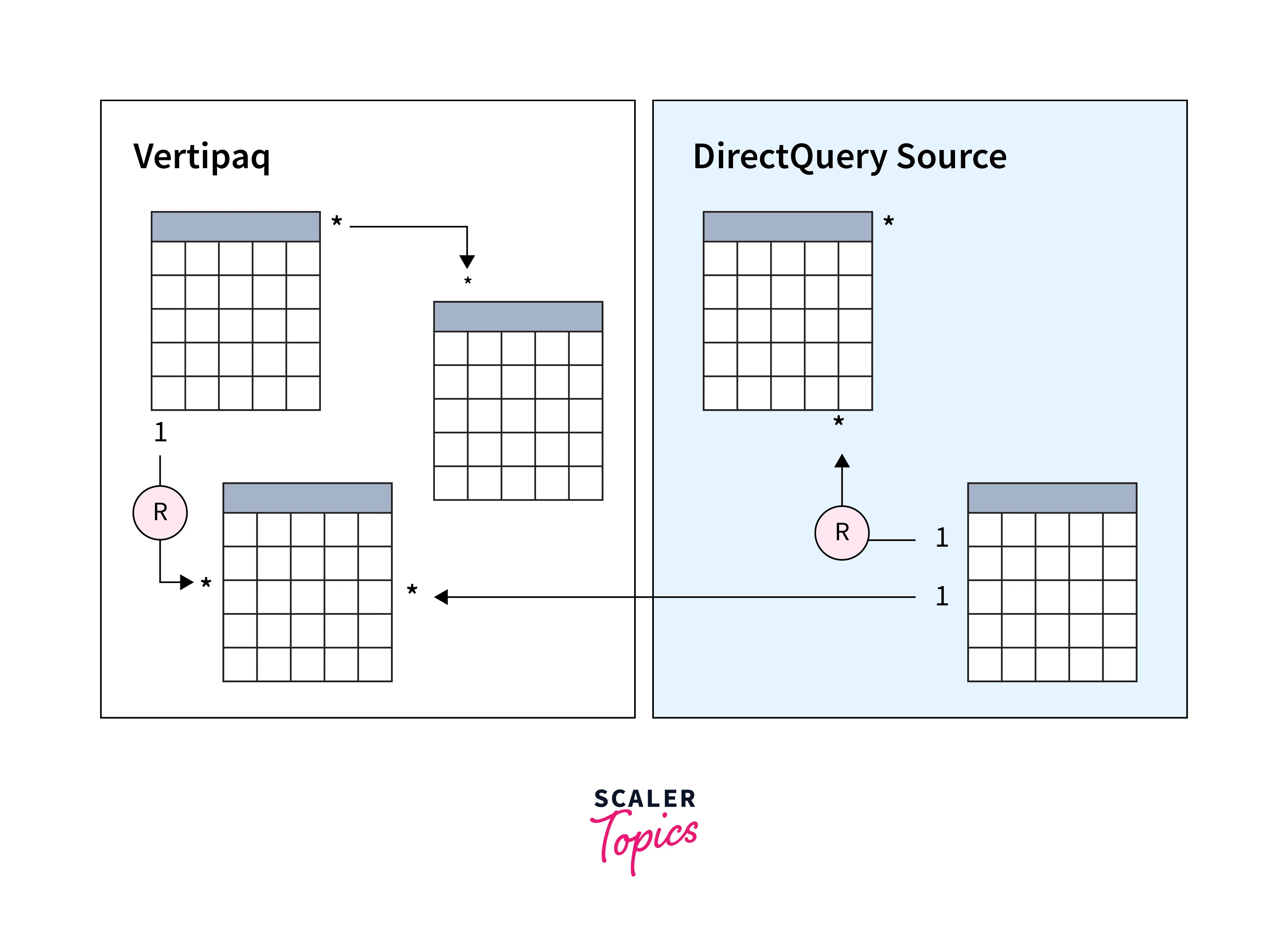
First, some modeling theory is needed to understand relationship evaluations. In an import or DirectQuery model, all data is sourced from either the Vertipaq cache or the source database, allowing Power BI to determine the existence of a "one" side in a relationship.
However, in a composite model, which can combine tables with different storage modes (import, DirectQuery, or dual) or multiple DirectQuery sources, each source forms a source group. Model relationships in a composite model can be classified as an intra-source group or inter/cross-source group. An intra-source group relationship relates tables within the same source group, while an inter/cross-source group relationship connects tables across different source groups. It's important to note that relationships in import or DirectQuery models are always considered intra-source group relationships.
For instance, consider a composite model consisting of two source groups - a Vertipaq source group with three tables and a DirectQuery source group with two tables. In this case, a cross-source group relationship exists to relate a table in the Vertipaq source group to a table in the DirectQuery source group.

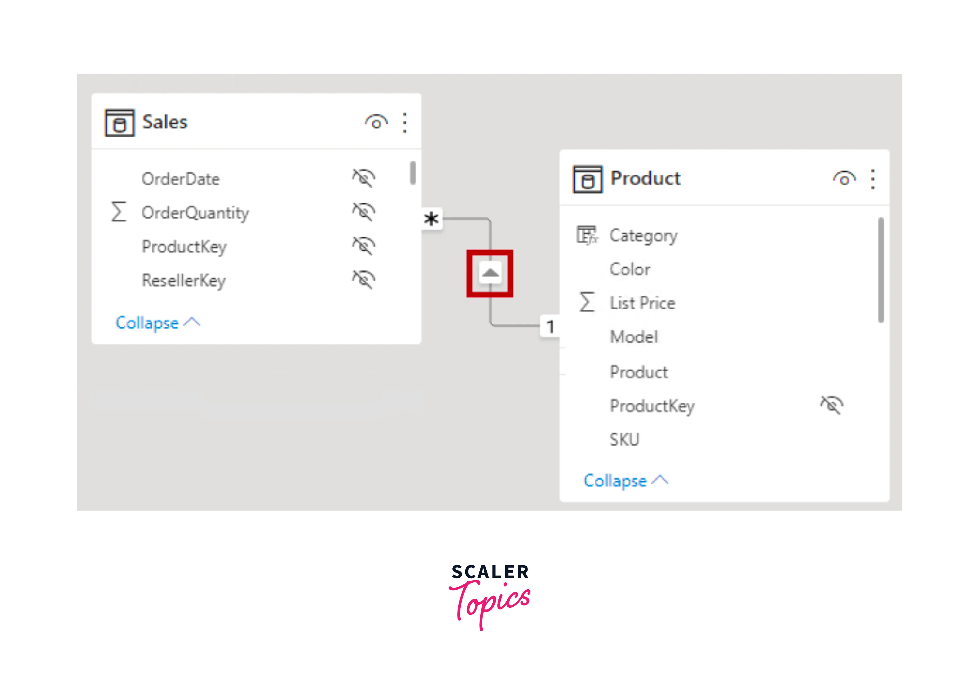
Regular Relationships
A model relationship is considered regular when the query engine can confirm the uniqueness of the "one" side column in the relationship. All one-to-many intra-source group relationships fall under the category of regular relationships. As shown in the below figure, there are two regular relationships marked as R.
For import models, where all data is stored in the Vertipaq cache, Power BI creates data structures for each regular relationship during data refresh. These data structures consist of indexed mappings of column-to-column values, aiming to accelerate table joins at query time.
At query time, regular relationships allow table expansion to occur. Table expansion involves creating a virtual table that includes native columns from the base table and then expands into related tables. This expanded table is then utilized by the query engine for filtering and grouping based on the values in the expanded table columns. It's important to note that inactive relationships are also expanded, regardless of whether they are used in calculations. However, bi-directional relationships do not impact table expansion.
For one-to-many relationships, table expansion occurs from the "many" to the "one" sides using LEFT OUTER JOIN semantics. If a matching value from the "many" to the "one" side doesn't exist, a blank virtual row is added to the "one" side table. This behavior applies specifically to regular relationships, not limited relationships. Table expansion also occurs for one-to-one intra-source group relationships, using FULL OUTER JOIN semantics. This join type ensures that blank virtual rows are added on either side when necessary.
Blank virtual rows represent unknown members and indicate referential integrity violations where a value from the "many" side has no corresponding value on the "one" side. Ideally, these blanks should be eliminated by cleansing or repairing the source data to maintain data accuracy and integrity.
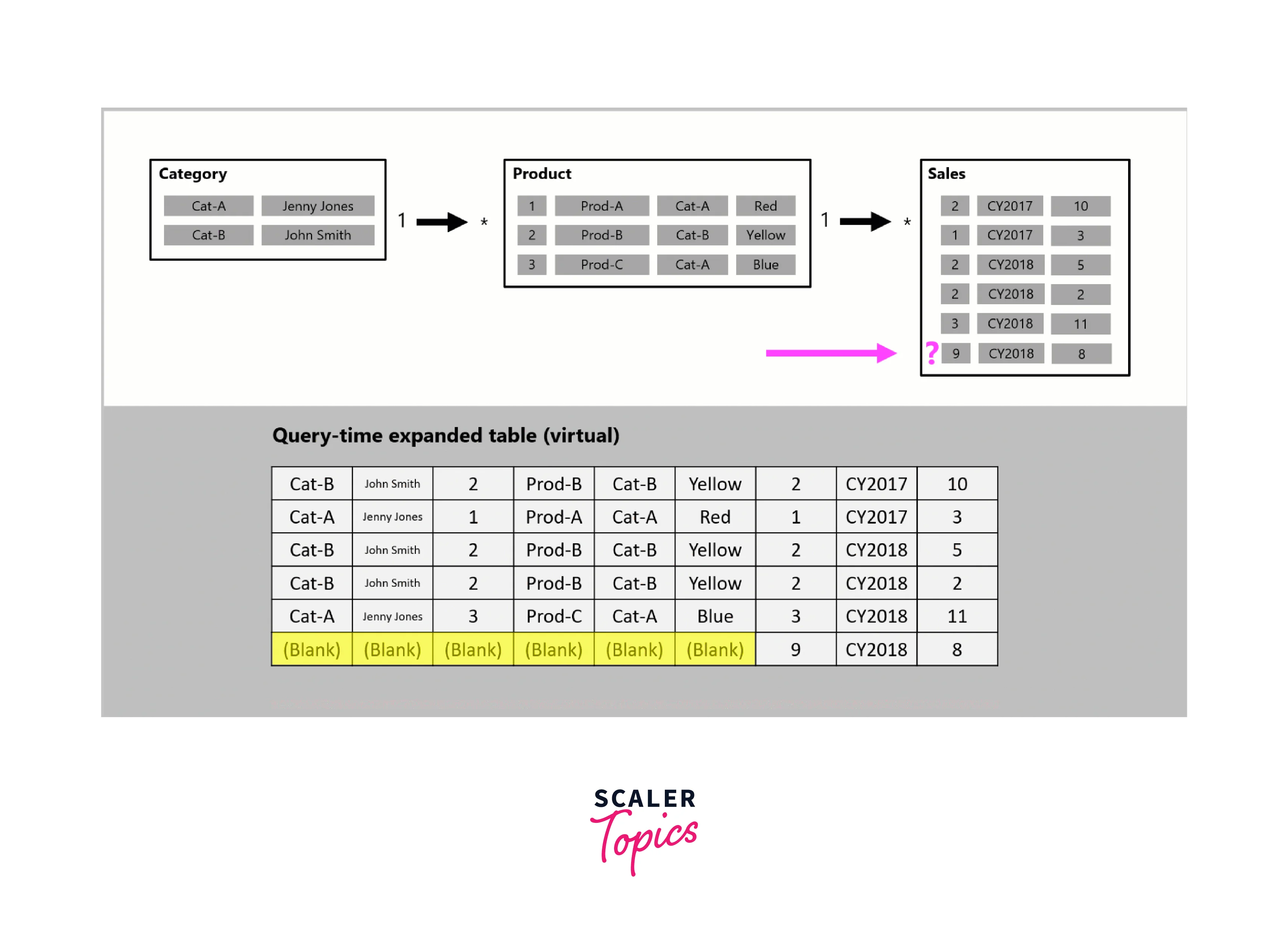
In the below figure, the data model comprises three tables - Category, Product, and Sales. A One-to-many relationship exists between the Category and Product tables, and another One-to-many relationship links the Product and Sales tables. The Category table holds two rows, the Product table contains three rows, and the Sales table contains five rows. Due to matching values on both sides of the relationships, there are no referential integrity violations.
Upon query execution, a query-time expanded table is generated, encompassing columns from all three tables. For instance, a new row is introduced in the Sales table, featuring a production identifier value (9) that has no corresponding match in the Product table. This situation represents a referential integrity violation. The new row displays (Blank) values in the Category and Product table columns in the expanded table.
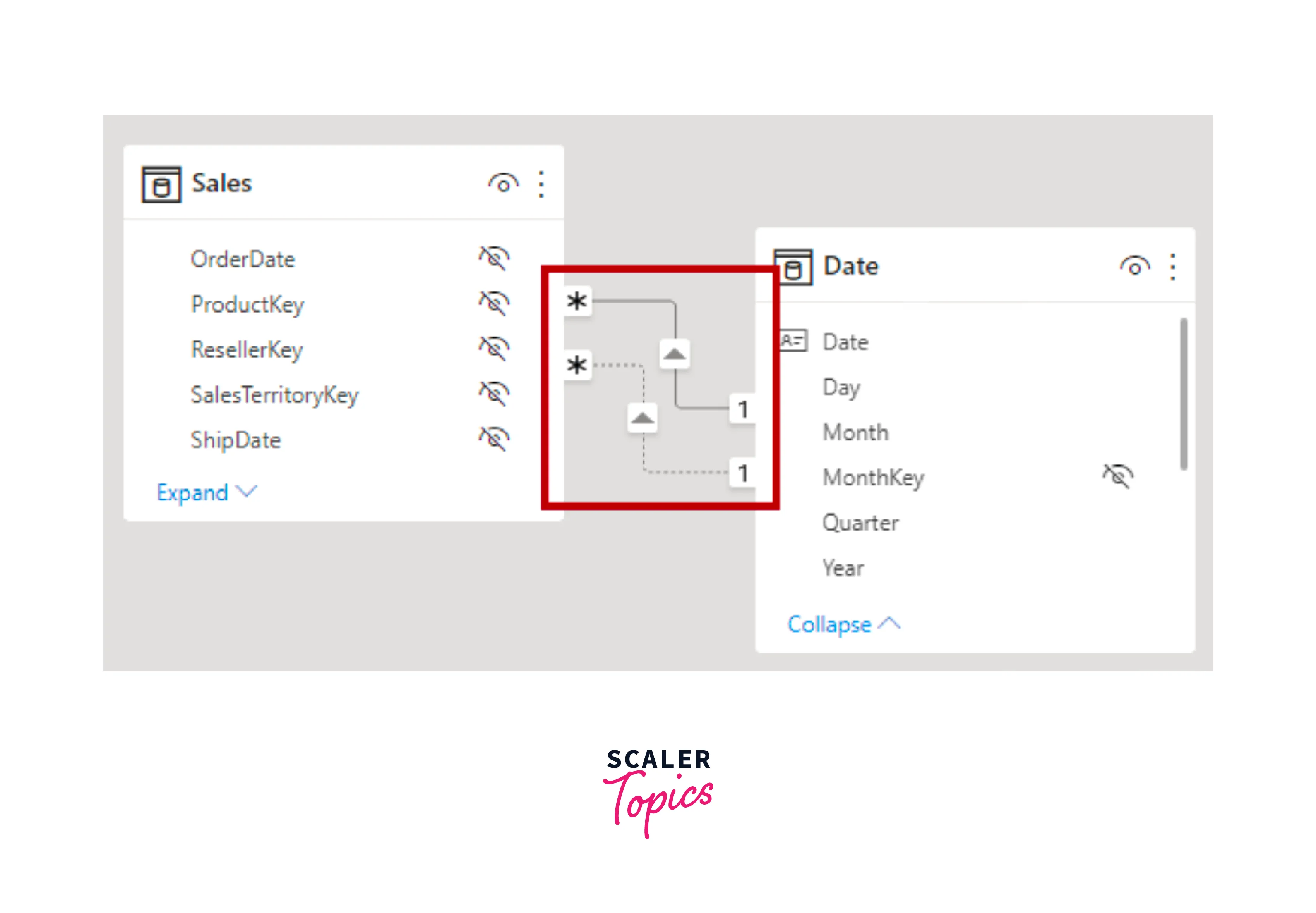
Limited Relationships
A model relationship is considered limited when there is no guaranteed "one" side in the relationship. There are two primary reasons why a relationship becomes limited -
- Many-to-Many Cardinality -
If the relationship involves a many-to-many type, even if one or both columns have unique values, the relationship becomes limited. - Cross Source Group -
Limited relationships can occur when dealing with composite models that involve tables from different source groups.
As shown in the figure below, there are two limited relationships marked as L. The two relationships include the many-to-many relationship within the Vertipaq source group and the one-to-many cross-source group relationship.

In import models, data structures are not created for limited relationships during data refresh. Instead, Power BI resolves table joins directly at query time.
Unlike regular relationships, table expansion does not occur for limited relationships. Table joins are performed using INNER JOIN semantics, and as a result, blank virtual rows are not added to compensate for referential integrity violations.
In Power BI Desktop's model view, you can identify a limited relationship by noticing parenthesis-like marks ( ) placed after the cardinality indicators representing the relationship. These marks signify that the relationship is limited, indicating no guaranteed "one" side in the relationship.

Resolve Relationship Path Ambiguity
Bi-directional relationships in Power BI can create multiple filter propagation paths between model tables, leading to potential ambiguity. When faced with ambiguity, Power BI determines the filter propagation path for use according to its priority and weight.
Priority
To address relationship path ambiguity, Power BI follows priority tiers, establishing a sequence of rules. These rules determine the path to be taken when filters flow from a source table to a target table. The priority rules are as follows -
- A path consisting of one-to-many relationships takes precedence.
- If no one-to-many path exists, a path with one-to-many or many-to-many relationships is considered.
- Next, a path consisting of many-to-one relationships is evaluated.
- If no clear path is found yet, a combination of one-to-many relationships from the source table to an intermediate table, followed by many-to-one relationships from the intermediate table to the target table, is considered.
- Similarly, a combination of one-to-many or many-to-many relationships from the source table to an intermediate table, followed by many-to-one or many-to-many relationships from the intermediate table to the target table, is explored.
- Any other remaining paths are evaluated as a last resort.
Weight
Each relationship in a path carries a weight, which is equal by default unless the USERELATIONSHIP function is utilized. The path weight is determined as the maximum weight among all relationships along the path. Power BI relies on these path weights to resolve ambiguity when multiple paths exist in the same priority tier. It prioritizes paths with higher weights while disregarding lower-priority paths.
The number of relationships in the path does not affect the weight. Instead, you can influence the weight of a relationship using the USERELATIONSHIP function. The weight is determined by the nesting level of this function call, with the innermost call receiving the highest weight.
Performance Preference
The performance of filter propagation in Power BI varies based on the type of relationships involved. Here is the list, ordered from fastest to slowest performance -
- One-to-many relationships within the same source group demonstrate the fastest filter propagation speed.
- Many-to-many relationships achieved using an intermediary table, involving at least one bi-directional relationship, come next in terms of performance.
- Many-to-many cardinality relationships exhibit moderate filter propagation speed.
- Cross-source group relationships have the slowest filter propagation performance.
Conclusion
- Power BI's cardinality of relationship is a fundamental aspect of building efficient data models, defining the connections between tables, and governing how filters propagate within the model.
- Implementing star schema design principles is highly recommended to ensure smooth filter propagation and manage relationships effectively, especially in complex models comprising both dimensions and fact tables.
- Understanding the various cardinality types, including one-to-many, many-to-one, one-to-one, and many-to-many, is crucial for defining the nature of relationships between tables and optimizing data analysis.
- Power BI provides a range of relevant DAX functions, such as RELATED, RELATEDTABLE, USERELATIONSHIP, CROSSFILTER, and more, enabling users to handle relationships, perform advanced calculations, and create virtual relationships when needed.
- By considering regular, limited, and bi-directional relationships, users can navigate relationship ambiguity and make informed decisions when designing data models, ultimately leading to accurate and insightful data analysis within Power BI. By following priority and weight rules, users can influence filter propagation paths and enhance the performance of their data models, ensuring a seamless and efficient user experience.