Logistic Regression in R

Introduction to Logistic Regression

Logistic regression is a widely used statistical method in machine learning and statistics that plays a crucial role in binary classification tasks. Unlike its linear regression counterpart, which predicts continuous numerical values, logistic regression is specifically designed for problems where the outcome is binary or categorical, such as predicting whether an email is spam or not, whether a patient has a disease or not, or whether a customer will purchase a product or not.

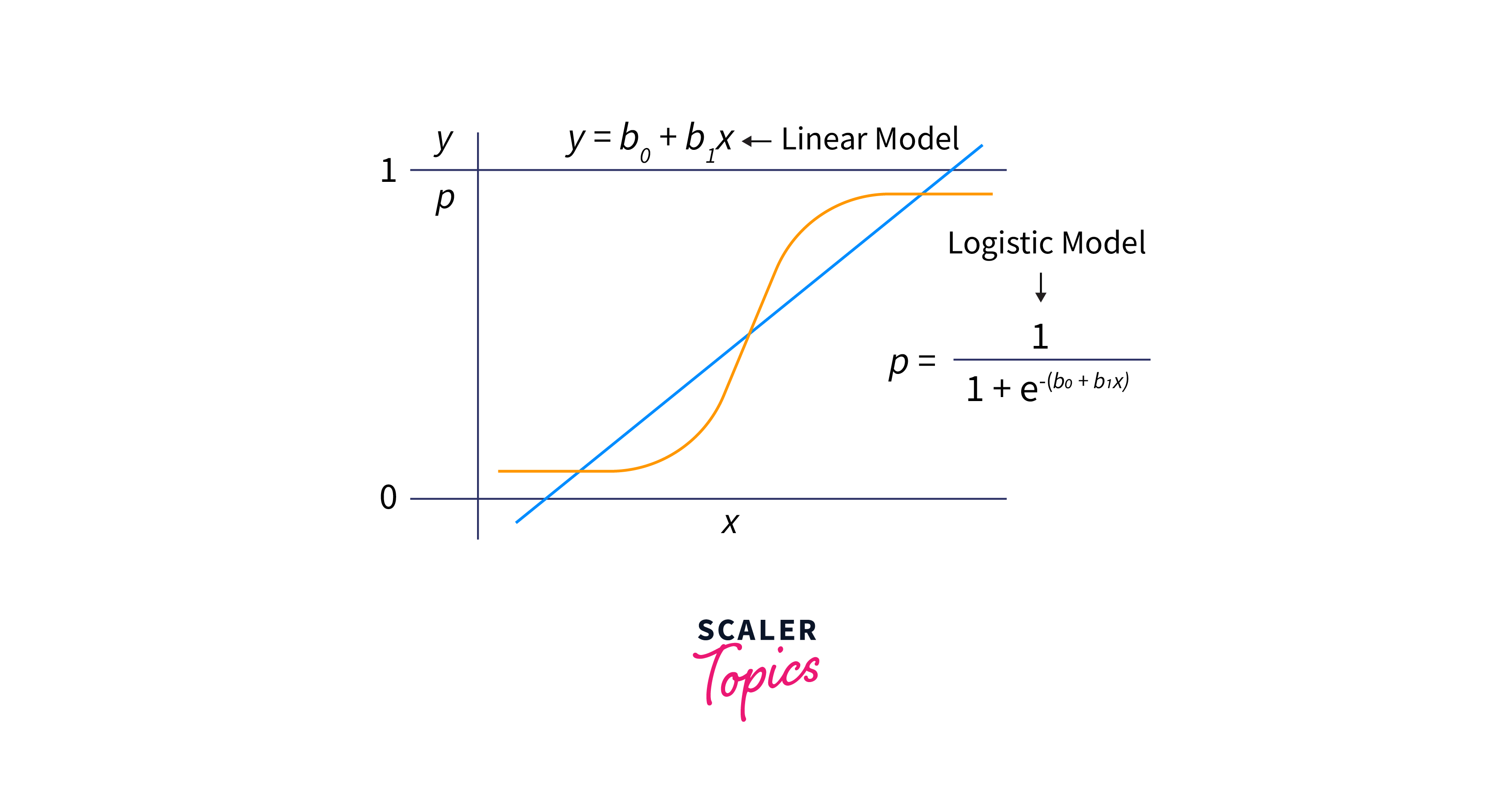
At its core, logistic regression models the probability that a given input instance belongs to one of the two possible classes. It achieves this by applying the logistic function (also known as the sigmoid function) to a linear combination of input features.

Now that we know the basics of logistic regression let us understand the theory behind logistic regression.

Theory behind Logistic Regression

Logistic regression is based on the logistic function, an S-shaped curve that maps any real-valued number to a value between 0 and 1. The logistic function is defined as:

In this formula:

• P(Y=1) represents the probability that the dependent variable Y belongs to class 1.
• z is the linear combination of predictor variables weighted by coefficients, typically represented as: z = β₀ + β₁X₁ + β₂X₂ + ... + βₚXₚ.
• e is the base of the natural logarithm, approximately equal to 2.71828.

Logistic regression models the log odds of the probability P(Y=1) as a linear combination of the predictor variables. The log-odds or logit is defined as:

The logistic function then converts the log odds into a probability value between 0 and 1.

Formula: The logistic regression formula for predicting the probability that an observation belongs to class 1 is:

Where z is calculated as:

In this formula:

• P(Y=1) is the predicted probability of belonging to class 1.
• X₁, X₂, ..., Xₚ are the predictor variables.
• β₀, β₁, β₂, ..., βₚ are the coefficients (parameters) associated with each predictor variable.
• 'e' serves as the natural logarithm's base.

The logistic regression model is trained by estimating the values of the coefficients (β₀, β₁, β₂, ..., βₚ) using a technique like maximum likelihood estimation. Once the model is trained, it can be used to predict probabilities for new input data and make binary classification decisions based on a chosen threshold (e.g., if P(Y=1) > 0.5, classify as class 1; otherwise, classify as class 0).

Implementation of Logistic Regression in R

Implementing logistic regression in R is straightforward, especially with the help of the built-in functions provided by R's glm (generalized linear model) function. Here's a step-by-step guide on how to implement logistic regression in R:

That's a basic overview of implementing logistic regression in R. Remember to preprocess your data, handle categorical variables, and perform feature engineering to improve model performance. Additionally, consider splitting your data into training and testing sets for model evaluation and validation.

Overview of Logistic Regression

In this section, we will use the mtcars dataset to implement logistic regression in R. After performing various steps of pre=processing; we will use the glm package to perform logistic regression.

Step 1: The Dataset

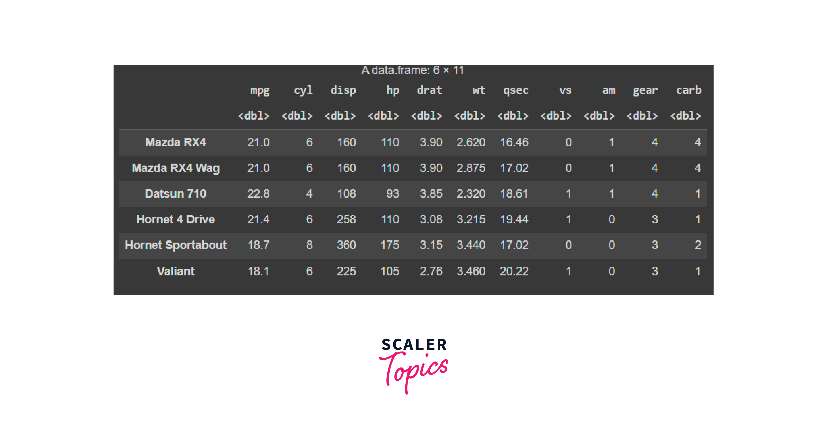
As discussed earlier, we will be using the mtcars package. mtcars is a built-in dataset in R that contains data on 32 different car models, with attributes like miles per gallon (mpg), horsepower (hp), and weight (wt). It's commonly used for data analysis and modeling tasks in R due to its simplicity and versatility, making it a valuable resource for learning and practicing data analysis techniques.

Output

Logistic Regression Workflow

The logistic regression workflow typically involves the following steps:

1. Data Preparation: Collect and clean your dataset, ensuring it's in a suitable format for analysis.
2. Data Visualization: Explore your data using visualizations to understand relationships and identify potential predictors.
3. Dataset Splitting: Divide your data into training and testing sets to assess model performance.
4. Model Building: Fit a logistic regression model to your training data, specifying the dependent and predictor variables.
5. Model Evaluation: Evaluate the model on the test data using metrics like accuracy, precision, recall, F1-score, ROC curves, and AUC.
6. Hyperparameter Tuning: Fine-tune model parameters (e.g., regularization strength) using techniques like cross-validation.

This workflow helps build, evaluate, and interpret logistic regression models for classification tasks, making it a valuable tool in various fields like healthcare, finance, and marketing.

Logistic Regression Packages

Here's the different packages used in this implementation:

1. dplyr:
   • dplyr is a powerful package for data manipulation and transformation. It provides functions like filter, select, and mutate to efficiently manipulate data frames.
2. ggplot2:
   • ggplot2 is a popular package for creating data visualizations using a grammar of graphics approach. It allows you to create highly customizable and publication-quality plots with ease.
3. caret:
   • caret (Classification And Regression Training) is a versatile package for machine learning in R. It provides a unified interface for training and evaluating various models, including logistic regression, while offering tools for hyperparameter tuning and resampling methods like cross-validation.
4. glmnet:
   • glmnet is used for fitting generalized linear models (GLMs) with L1 and L2 regularization (i.e., Lasso and Ridge regression). It's particularly useful for logistic regression when controlling overfitting and selecting important features by tuning the regularization parameters (alpha and lambda).

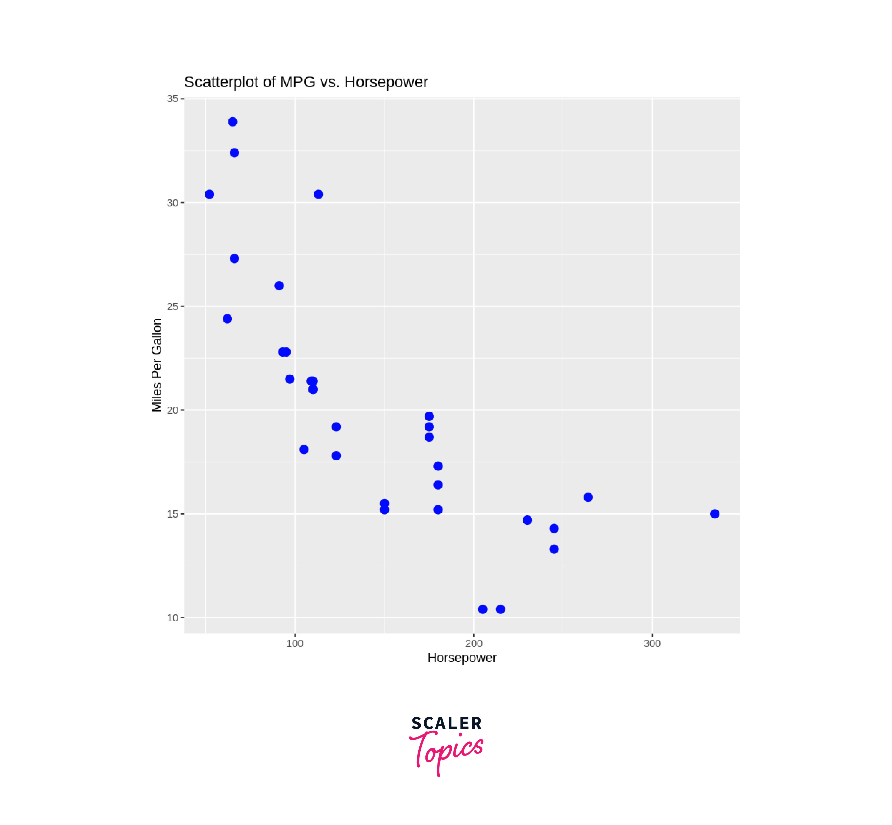
Step 2: Visualize the Data

We will visualize our dataset using the ggplot2 package in R.

Output

Step 3. Splitting the Data

We will split the data into training and testing sets to train our model.

Step 4. Fitting and Evaluating the Model

Output

Step 5: Hyperparameter Training

Using grid search, we will perform hyperparameter tuning for this dataset.

Output

More Evaluation Metrics

In addition to accuracy, Other evaluation measures that are frequently used to rate the effectiveness of R's logistic regression models. Here are a few key ones:

1. Confusion Matrix: The breakdown of true positive (TP), true negative (TN), false positive (FP), and false negative (FN) predictions is given in a confusion matrix. You can create it using the confusionMatrix function from the caret package.

2. Precision: Precision assesses the fraction of correct positive predictions relative to all positive predictions. It is useful when minimizing false positives is critical.

3. Recall (Sensitivity): Recall (Sensitivity) measures the proportion of true positives among all actual positives. It is crucial when minimizing false negatives is important.

4. F1-Score: The harmonic mean of recall and precision is the F1-score. It balances the trade-off between false positives and false negatives.

5. Receiver Operating Characteristic (ROC) Curve: The ROC curve plots the true positive rate (TPR or recall) against the false positive rate (FPR) at various thresholds. You can calculate it using the roc function from the pROC package and compute the area under the curve (AUC) to quantify model performance.

6. Area Under the ROC Curve (AUC): AUC quantifies the overall performance of a logistic regression model. A higher AUC indicates better discrimination between positive and negative cases.

7. Log-Loss (Cross-Entropy Loss): Log-loss measures the accuracy of predicted probabilities. Lower values indicate better model calibration. You can calculate it using the logLoss function from the Metrics package.

These evaluation metrics provide a comprehensive view of the performance of your logistic regression model, helping you assess its strengths and weaknesses for classification tasks.

Applications of Logistic Regression

As discussed earlier, logistic regression is a statistical technique used for binary classification problems where the outcome variable is categorical and has only two possible values (typically 0 and 1). Here are four common applications of logistic regression:

1. Medical Diagnosis: Logistic regression is widely used in the medical field for tasks such as disease diagnosis. For example, it can be used to predict whether a patient has a particular disease (1) or does not have it (0) based on various medical test results and patient characteristics. It's also used for predicting the likelihood of surgical complications, mortality risk, or the presence of a particular medical condition.

2. Marketing and Customer Analytics: Logistic regression helps predict customer behavior in marketing. It can predict whether a customer will likely buy a product (1) or not (0) based on factors like demographic information, past purchase history, and website interactions. This data can be used by marketers to efficiently target particular customer categories and customize their marketing tactics.

3. Credit Scoring: Logistic regression is frequently employed in the finance industry for credit scoring and risk assessment. Lenders use logistic regression models to predict the probability of a borrower defaulting on a loan (1) or repaying it (0). This information is crucial for determining creditworthiness and setting interest rates for loans.

4. Employee Attrition Prediction: In human resources and workforce management, logistic regression can predict employee turnover. Organizations can create models to forecast whether an employee will leave the company (1) or stay (0) by looking at aspects like job satisfaction, income, work hours, and employee demographics. This helps in identifying high-risk employees and implementing retention strategies.

These are just a few examples of the many applications of logistic regression. It is a versatile tool for binary classification tasks across various domains where understanding and predicting categorical outcomes is important.