Regularization in Machine Learning

What are Overfitting and Underfitting?

Before diving into regularization, let's clarify the concepts of overfitting and underfitting.

Overfitting:

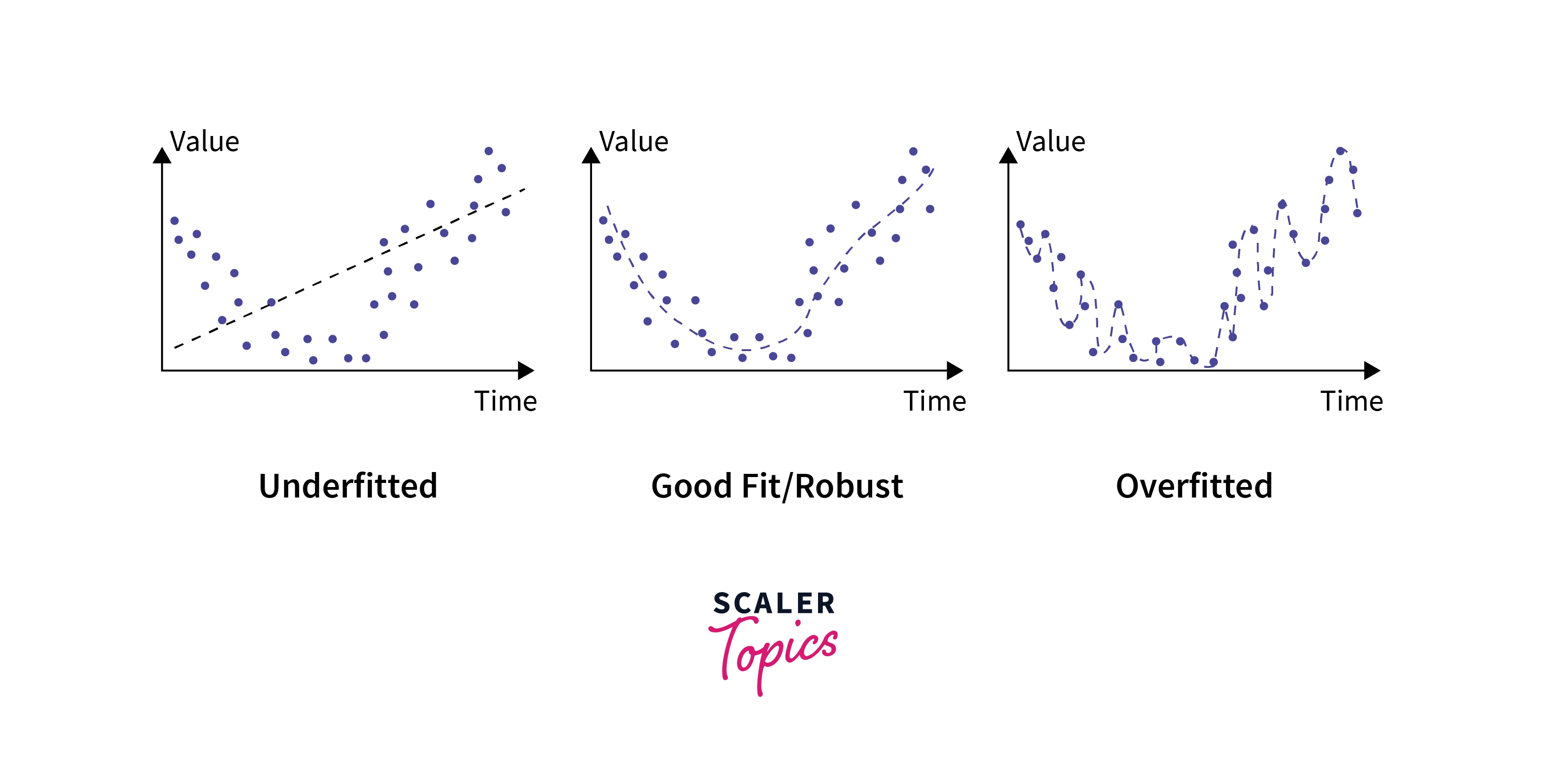
This occurs when a machine learning model learns the training data too well. In other words, the model becomes so flexible that it captures the noise and outliers in the training data, rather than the underlying patterns. As a result, it performs exceptionally well on the training data but poorly on new, unseen data.

Underfitting:

In contrast, underfitting happens when a model is too simplistic to capture the underlying patterns in the data. It performs poorly on both the training data and new data because it fails to learn the essential relationships.

Learn more about Overfitting and Underfitting in Machine Learning

What are Bias and Variance?

Bias and variance are two key concepts closely related to overfitting and underfitting:

Bias:

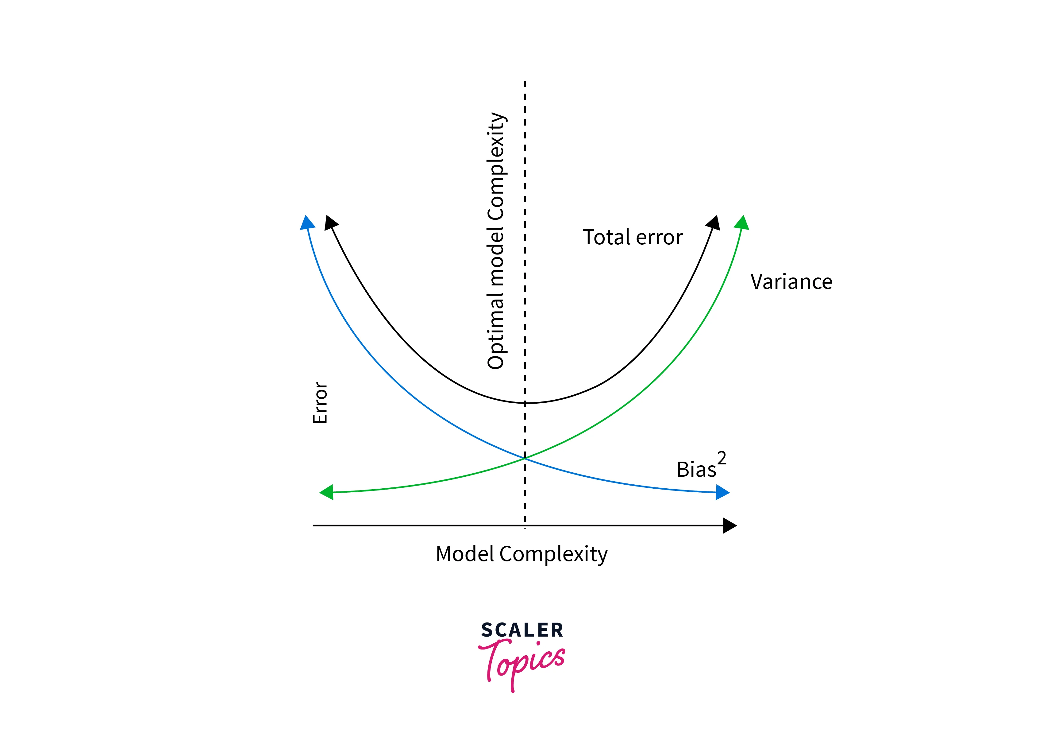
Bias measures how far off the predictions of a model are from the actual values. High bias indicates that the model is too simple and is underfitting the data.

Variance:

Variance quantifies the model's sensitivity to small changes in the training data. High variance suggests that the model is too complex and is overfitting the data.

Let's understand this with an example:

Bias: Think of a model with high bias as a chef who only knows how to make one simple dish, like scrambled eggs. No matter what ingredients you give them, they'll always make scrambled eggs. This chef is inflexible and can't adapt to different tastes or recipes.

Variance: Now, imagine a different chef with high variance. This chef can cook many complex dishes, but they are very inconsistent. Sometimes they make a fantastic gourmet meal, and other times they create a disaster because they keep trying new, risky recipes without sticking to what they know works.

So, the goal in machine learning is to find a chef (model) who can learn to cook a variety of dishes (make predictions on different data) but doesn't always stick to just one (low bias) and also doesn't go wild experimenting all the time (low variance). You want a balanced chef who can adapt and consistently make delicious meals (accurate predictions).

Achieving the right balance between bias and variance is essential for building a robust machine learning model, and this is where regularization comes into play.

What is Regularization in Machine Learning?

Regularization is a technique used to prevent overfitting and control model complexity. It adds a penalty term to the loss function that the model aims to minimize during training. This penalty discourages the model from assigning excessively large coefficients to the input features.

There are two widely used types of regularization in machine learning:

L1 Regularization

L1 regularization, also known as Lasso regularization, adds the absolute values of the coefficients as a penalty term to the loss function. Mathematically, it adds the sum of the absolute values of the coefficients to the loss function.

The L1 regularization term can be represented as:

Where:

• $L1$ is the $L1$ regularization term.
• $\lambda$ is the regularization parameter, controlling the strength of regularization.
• $w_i$ represents the coefficients of the model.

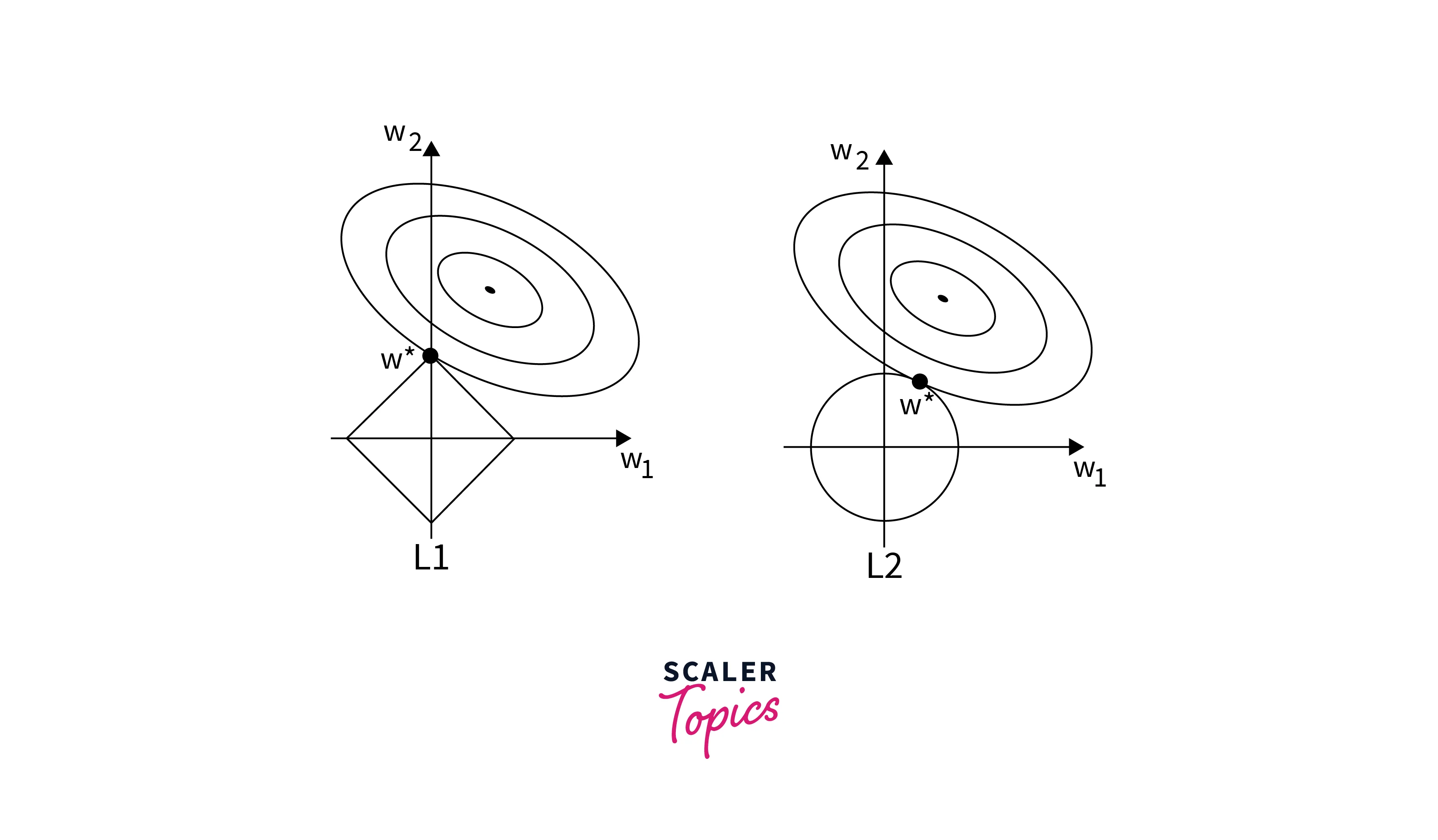
L1 regularization has a unique property: it can drive some of the coefficients to exactly zero. This feature makes it useful for feature selection, as it effectively removes irrelevant features from the model.

L2 Regularization

L2 regularization, also known as Ridge regularization, adds the squared values of the coefficients as a penalty term to the loss function. Mathematically, it adds the sum of the squared values of the coefficients to the loss function.

The L2 regularization term can be represented as:

Where:

• $L2$ is the $L2$ regularization term.
• $\lambda$ is the regularization parameter, controlling the strength of regularization.
• $w_i$ represents the coefficients of the model.

Unlike L1 regularization, L2 regularization does not drive coefficients to zero but shrinks them towards zero. This helps in reducing the magnitude of the coefficients and, consequently, the model's complexity.

How Does Regularization Work?

Regularization techniques like L1 and L2 work by adding a penalty term to the loss function that the model aims to minimize. This penalty term discourages the model from having large coefficients. Here's how it works:

• The loss function consists of two components: the data loss (how well the model fits the training data) and the regularization term (the penalty for large coefficients).
• During training, the model aims to minimize this combined loss function.
• The regularization parameter $\lambda$ controls the trade-off between fitting the data well and keeping the coefficients small.
• As the regularization parameter $\lambda$ increases, the impact of the regularization term becomes more significant, forcing the model to have smaller coefficients.

Let's take a closer look at Lasso and Ridge Regression, two popular regularization techniques

Lasso Regression

Lasso Regression, which employs L1 regularization, is particularly effective when dealing with high-dimensional data with many irrelevant features. It tends to drive the coefficients of irrelevant features to exactly zero, effectively removing them from the model.

Lasso Regression is useful for feature selection because it automatically identifies and retains the most relevant features while discarding the rest. This can simplify the model and improve its interpretability.

Ridge Regression

Ridge Regression, on the other hand, uses L2 regularization and is effective in preventing multicollinearity, a situation where two or more features in a dataset are highly correlated. Multicollinearity can lead to unstable and unreliable coefficient estimates.

Ridge Regression adds a penalty term that encourages the model to distribute the coefficient values more evenly, reducing their magnitude. This results in a more stable and robust model.

Difference between Lasso Regression and Ridge Regression

While both Lasso and Ridge Regression are regularization techniques that add penalty terms to the loss function, they have key differences:

1. Type of Regularization Term:
   Lasso uses L1 regularization, which adds the absolute values of coefficients, while Ridge uses L2 regularization, which adds the squared values of coefficients.
2. Effect on Coefficients:
   Lasso tends to drive some coefficients to exactly zero, effectively performing feature selection. Ridge shrinks coefficients towards zero but does not force them to zero.
3. Use Cases:
   Lasso is useful when you suspect that many features are irrelevant, and you want to perform feature selection. Ridge is useful when you want to control multicollinearity and stabilize coefficient estimates.
4. Interpretability:
   Lasso can lead to a more interpretable model by selecting a subset of relevant features. Ridge does not perform feature selection and retains all features.

Regularization Using Python in Machine Learning

Now that we understand the theory behind regularization, let's see how to implement Lasso and Ridge Regression in Python using the popular machine learning library, scikit-learn.

Implementing Lasso Regression in Python

Implementing Ridge Regression in Python

In these examples, we use scikit-learn's Lasso and Ridge classes to create Lasso and Ridge Regression models, respectively. The alpha parameter controls the strength of regularization, with higher values leading to stronger regularization.