Understanding Recurrent Neural Networks

Introduction

Recurrent Neural Networks (RNNs) are a type of neural network designed to process sequential data, such as time series, text, or speech. One of the key features of RNNs is that they have "memory" in the form of hidden states, which allow the network to maintain information from previous time steps and use it to inform its predictions or decisions at later time steps.

An RNN comprises a series of repeating neural network "cells" that are connected in a chain-like structure, where the output of one cell is passed as input to the next cell. Each cell inputs the current input to the network and the hidden state from the previous time step, producing an output and a new hidden state. The hidden state is typically a fixed-size vector, and it is the key to the network's ability to maintain information from previous time steps.

Understanding a Recurrent Neural Network

Now, let us delve deeper into the rnn architecture. Take a look at the image below.

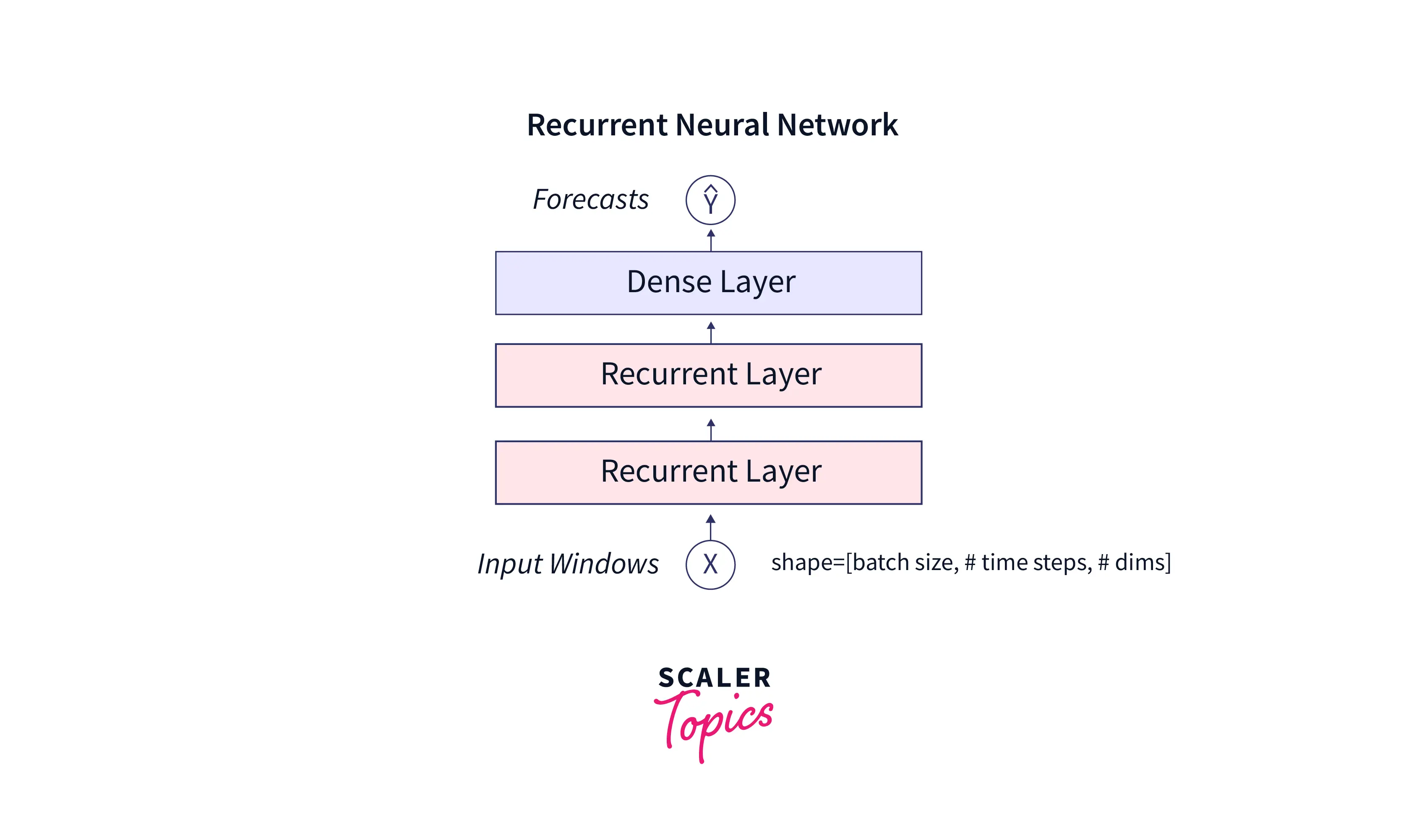
An rnn architecture generally takes a 3-dimensional input, namely batch size, the number of timesteps, and dimensions(can be univariate or multivariate). There can be many recurrent layers, as sown in the above image. Finally, for prediction, there will be a dense layer.

Take a look at the image below.

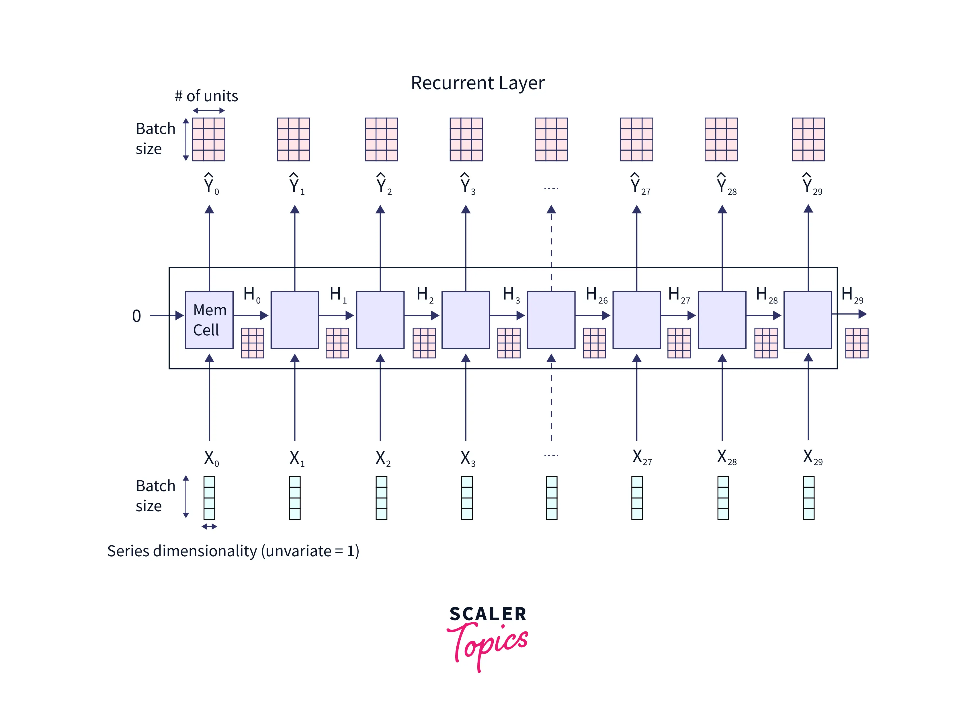
In the above image,

• $X_0, X_1,...... X_{29}$ are the different timesteps.
• The blue colored boxes are the inputs at different timesteps.
• Each "MemCell" constitutes the hidden layer.
• The orange boxes at the top of the image constitute the units of the hidden layer($3*3$ in the above case).
• It is important to note from the above image that $Y_0 = H_0$, $Y_1 = H_1$, and so on…
• To predict the output at a timestep, we must pass the hidden layer through a dense layer. We will see that next.

Now, Take a look at the image below.

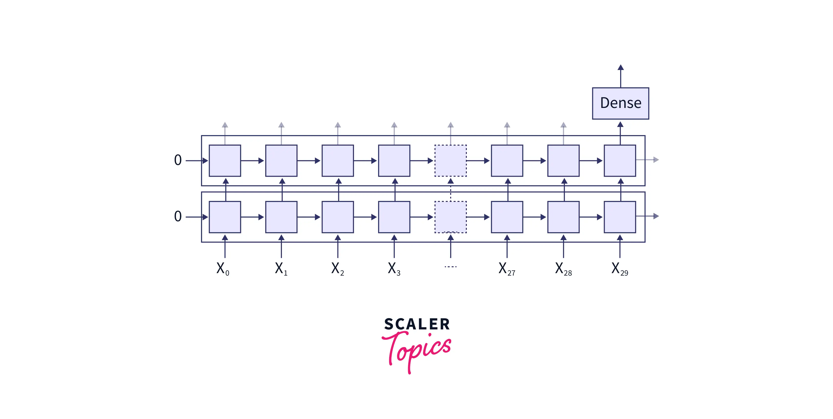
As we can see from the above image, there are two recurrent layers and one dense layer. For simplicity, we shall deal with the prediction of the word problem. We have the data for the first 29 timesteps(i.e., the first 29 words). Our task is to predict the word at the 30th timestamp. So we need to pass the hidden layer of the rnn architecture in the $X_{29}$ timestep through a dense layer to predict the output at the $X_{30}$(30th) timestep.

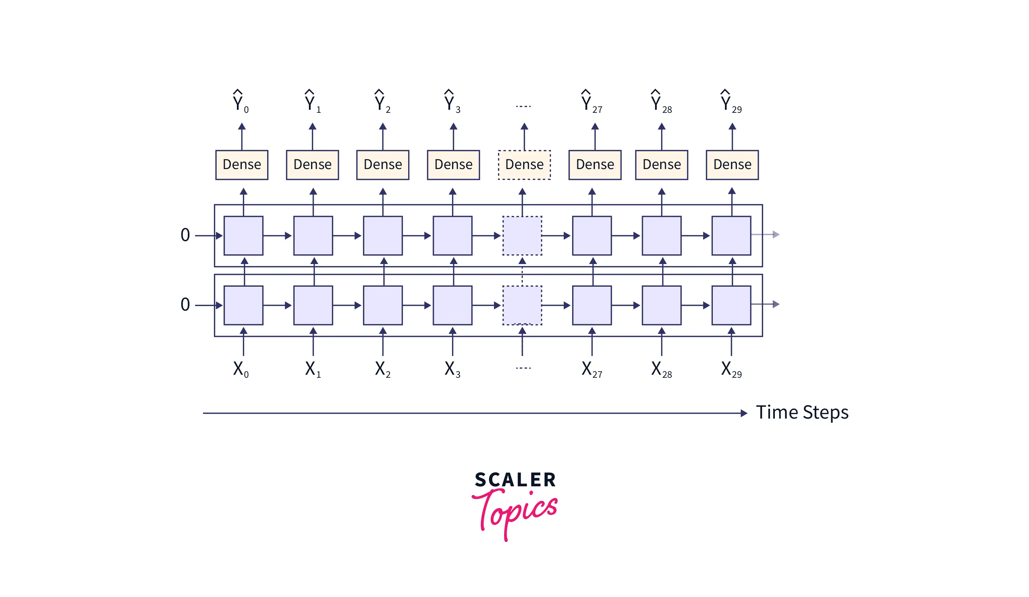
If we need to predict the output at each timestep, we must modify the rnn network architecture as below. Here $Y_{i}$ is the output at each timestep.

Now, a question arises - "How does the rnn architecture predict and learn stuff ?". We got this covered. This is what we will be looking into next.

Forward Propagation

Let us see how the forward propagation in an rnn architecture happens. Please take a deep look at the architecture above and then proceed further.

We know that the rnn architecture takes the current input value and the previously hidden layer as input to maintain and keep track of the state of the network. So, let us look at the following formulas, which will help us understand the rnn architecture better.

The formula to compute the values for the current hidden layer will depend on the current: input and previously hidden layer.

$h_t=\tanh \left(W_{h h} h_{t-1}+W_{x h} x_t\right)$

Here,

• $h_t$ = Current hidden layer
• $h_{t-1}$ = previous hidden layer
• $x_t$ = Current input
• $W_{hh}$ = Weights associated with the hidden layer(These are tuned while learning)
• $W_{x h}$ = Weights associated with the current input(These are tuned while learning)
• $tanh$ = The activation function

The formula to compute the output depends on the current hidden layer. It is given as follows:

$y_t=W_{h y} h_t$

Here,

• $y_t$ = Output
• $h_t$ = Current Hidden layer
• $W_{h y}$ = Weights associated with the current hidden layer(These are tuned while learning)

Using these formulas, the network gets fine-tuned and trained. Let's see how:

Let us consider this example. We are given the vocabulary 'h', 'e', 'l', 'l', and the word "hell". We must make the network predict the next letter after "he".

• First, we need to encode the input one-hot as follows:

  

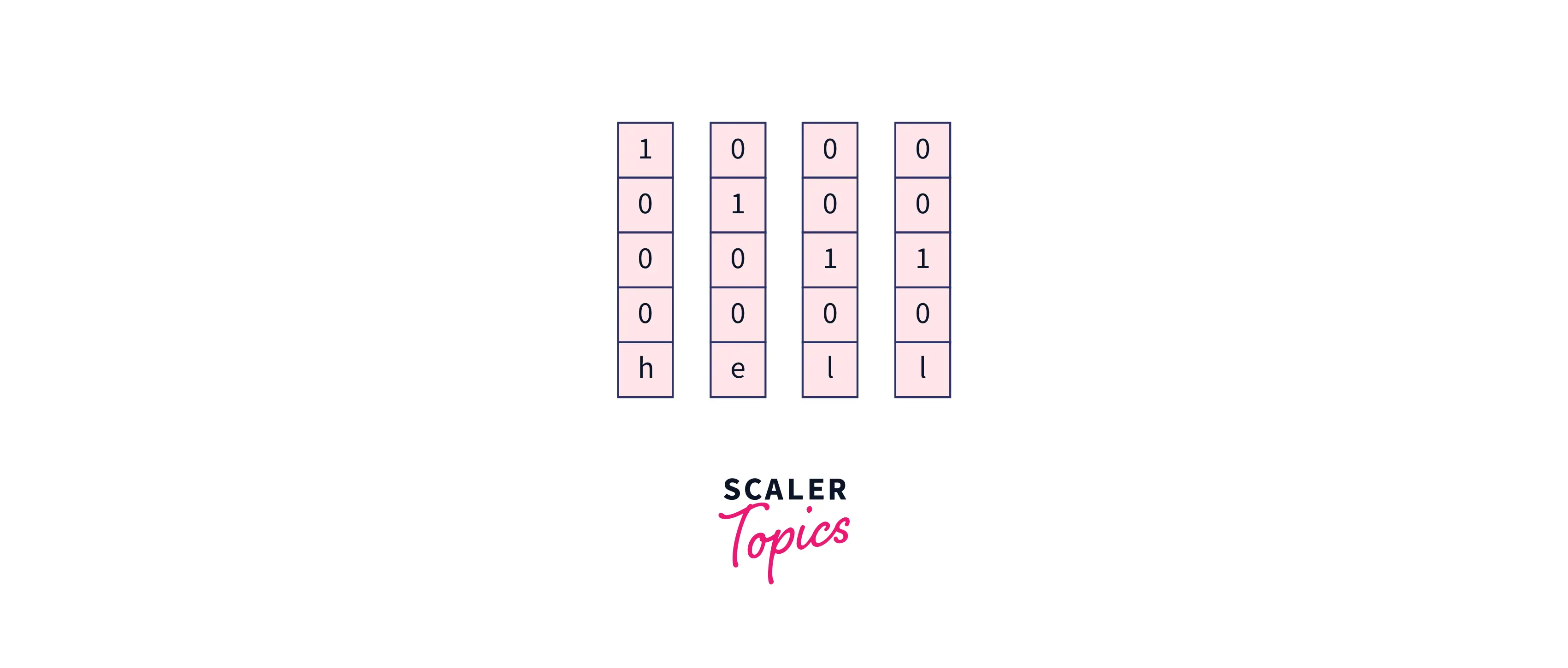
• Initialize $W_{xh}$

  

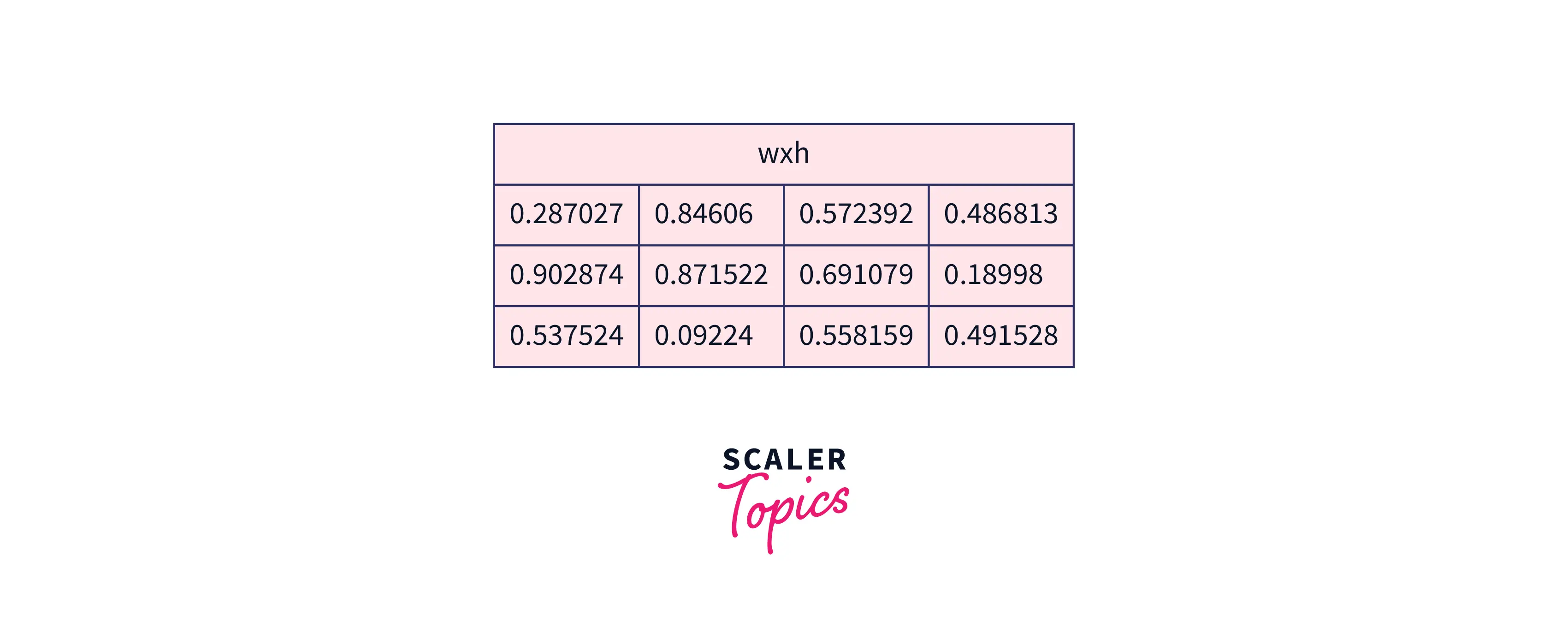
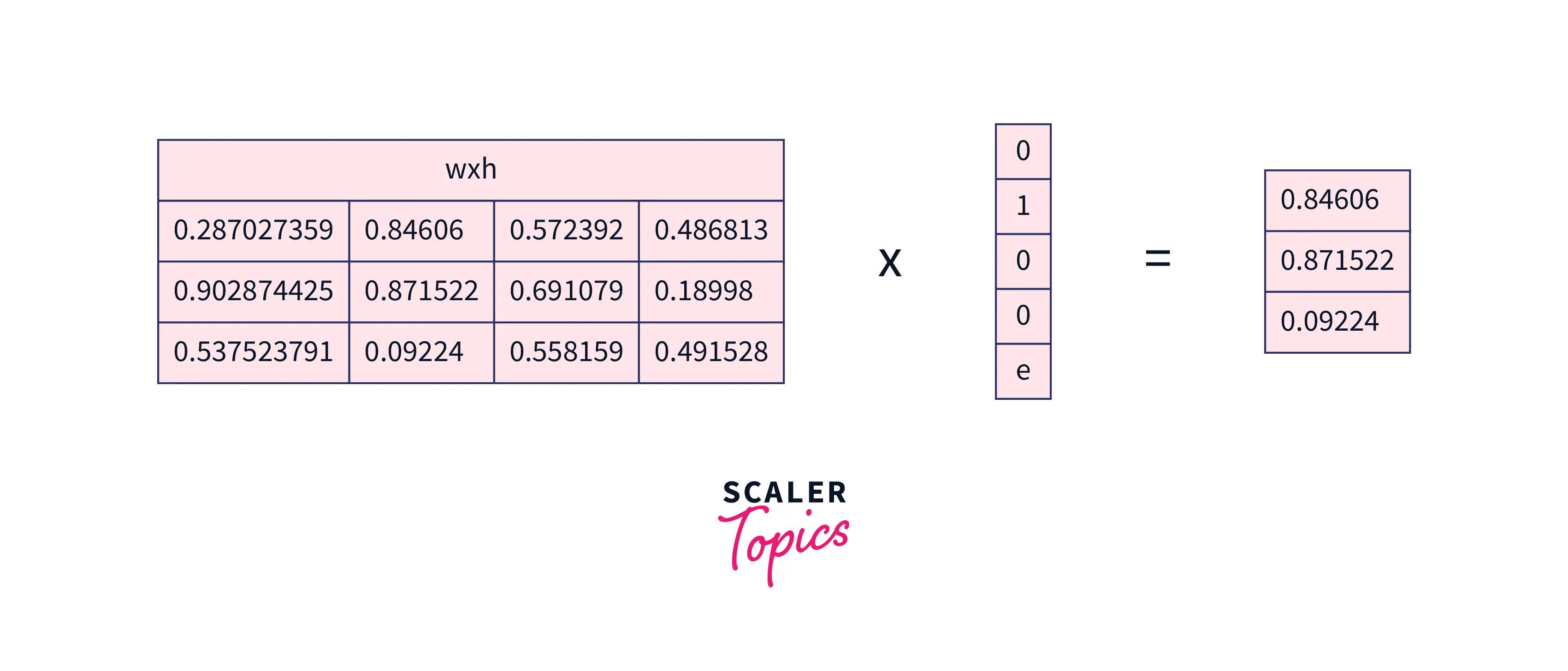
• Compute $W_{xh} * X_t$(curren tinput, in our case it is ‘h’):

  

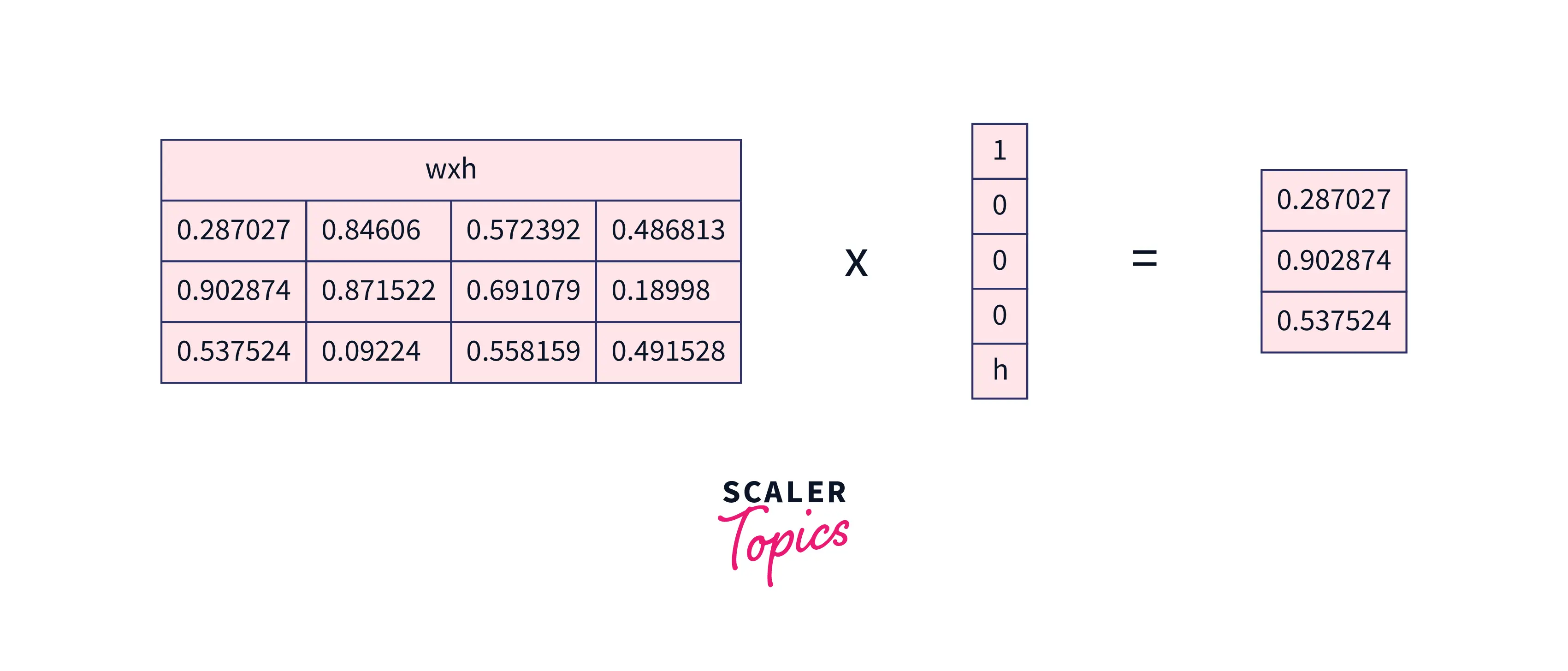
• Now, compute $W_{hh} * h_{t-1}$ and add some bias to it. We will assume Whh and the bias to be a $1*1$ matrix for simplicity. In the first case, $h_{t-1}$ will be all 0's as there will be no hidden layer before the hidden layer of the input $h$.

  

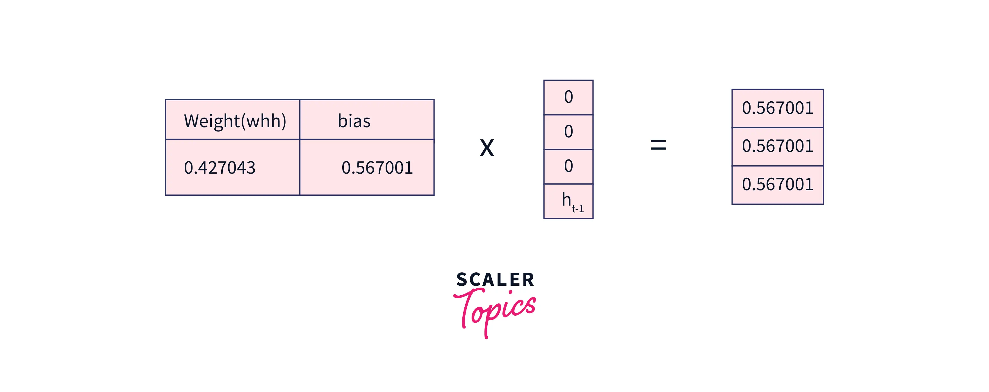
• Now, let us calculate the current hidden layer value using the currently hidden layer formula we saw above.

  

• In the next state, "e" is supplied to the network. $h_t$ will now become $h_{t-1}$, while the one hot encoded $e$ becomes $x_t$. Let us calculate the current state $h_t$ for "e". $W_{hh} * h_{t-1} + bias$ will be as follows:

  

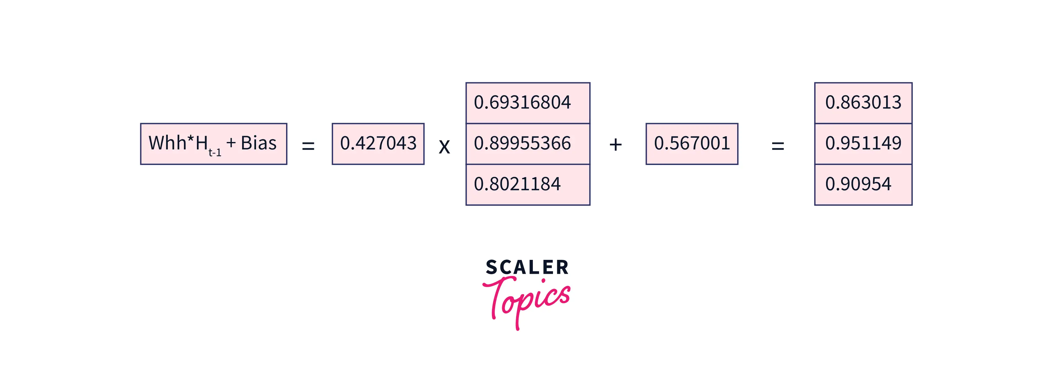
• $W_{xh} * x_t$ will be as follows:

  

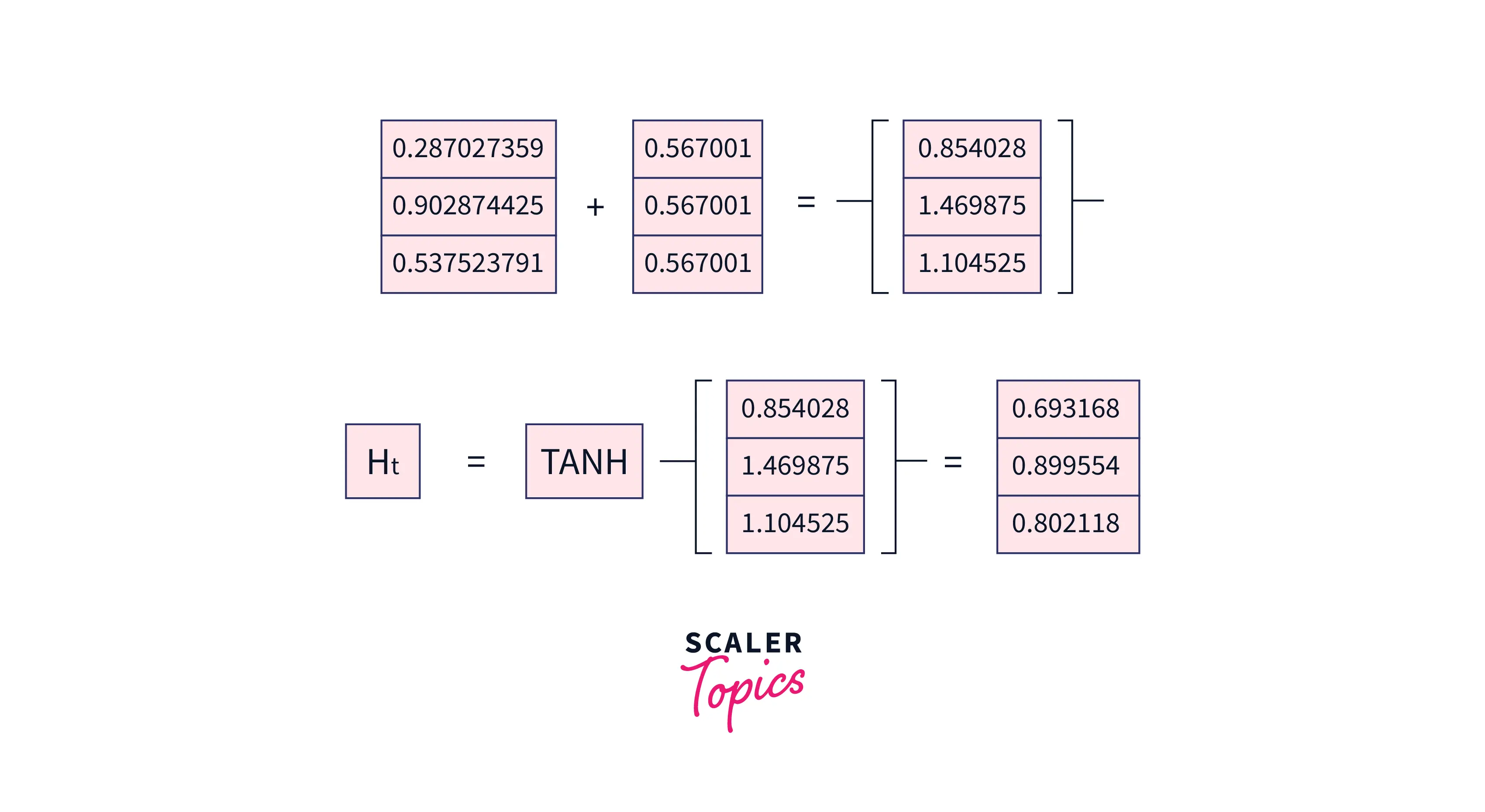
• Now, the hidden layer $h_t$ of "e" is as follows:

  

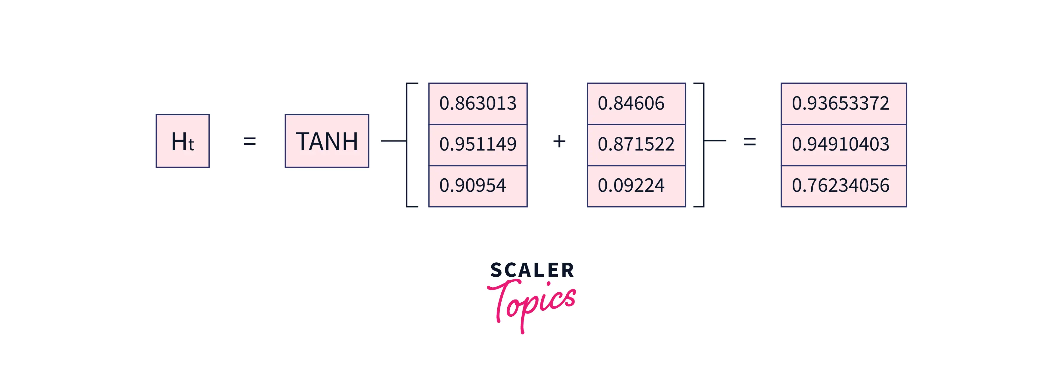
• Now, let us try to predict the next letter after "e" using the output formula $y_t$ given above.

  

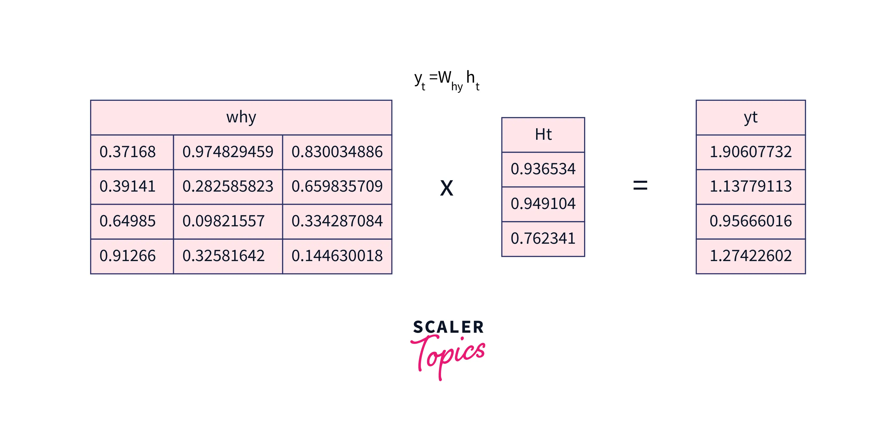
• Now, let's send $y_t$ through a softmax layer prediction of the next letter.

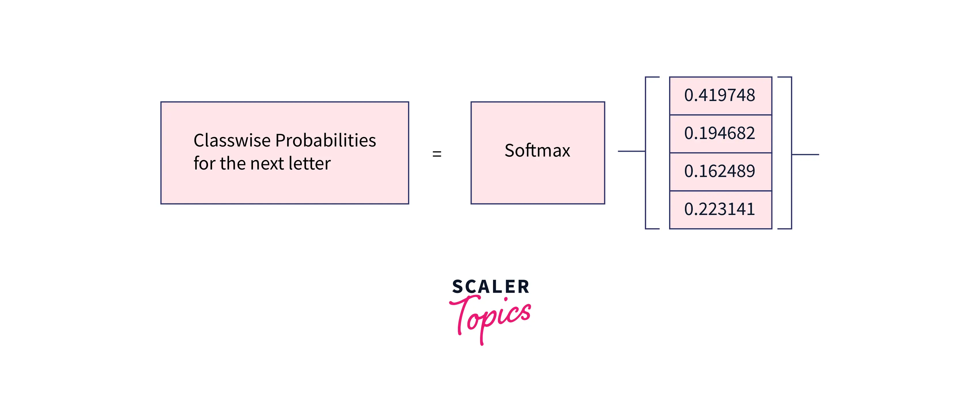
Since our vocabulary is limited to 'h', 'e', 'l', and 'l', from the above image, it is clear that the network predicts the next letter to be 'h' with $0.419748$ probability. (but 'l' should have been the prediction)

Yes, the network predicted wrongly. That is because the network needs to be more well-trained. The weights need to be tuned properly. Backpropagation through time improves performance, fine-tuning the weights and biases and improving the network's prediction. This is what we will see next.

Backpropagation through Time

Take a look at the image below.

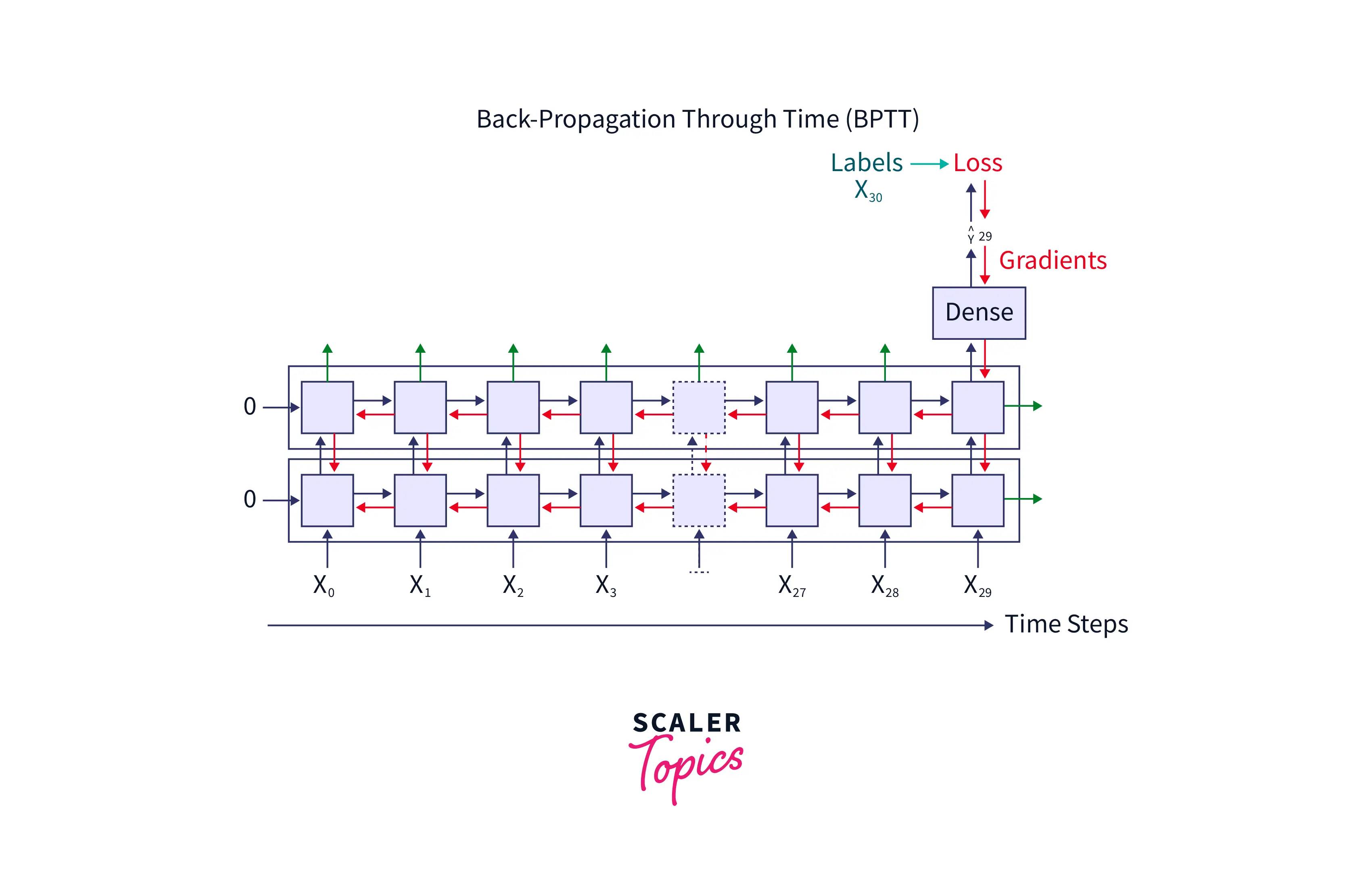
The above image shows that whenever the network predicts wrongly, it compares it with the original label, and the loss is propagated throughout the network. This happens until all the weights' values are identified so that the value of the loss function used to compute the loss is minimum. During this time, the weights and biases associated with the hidden layers and the input are fine-tuned.

Let us see how a single value of weight is fine-tuned in the rnn network with the help of an example below.

Let us generalize the concept for one variable; let's call it $θ1$.

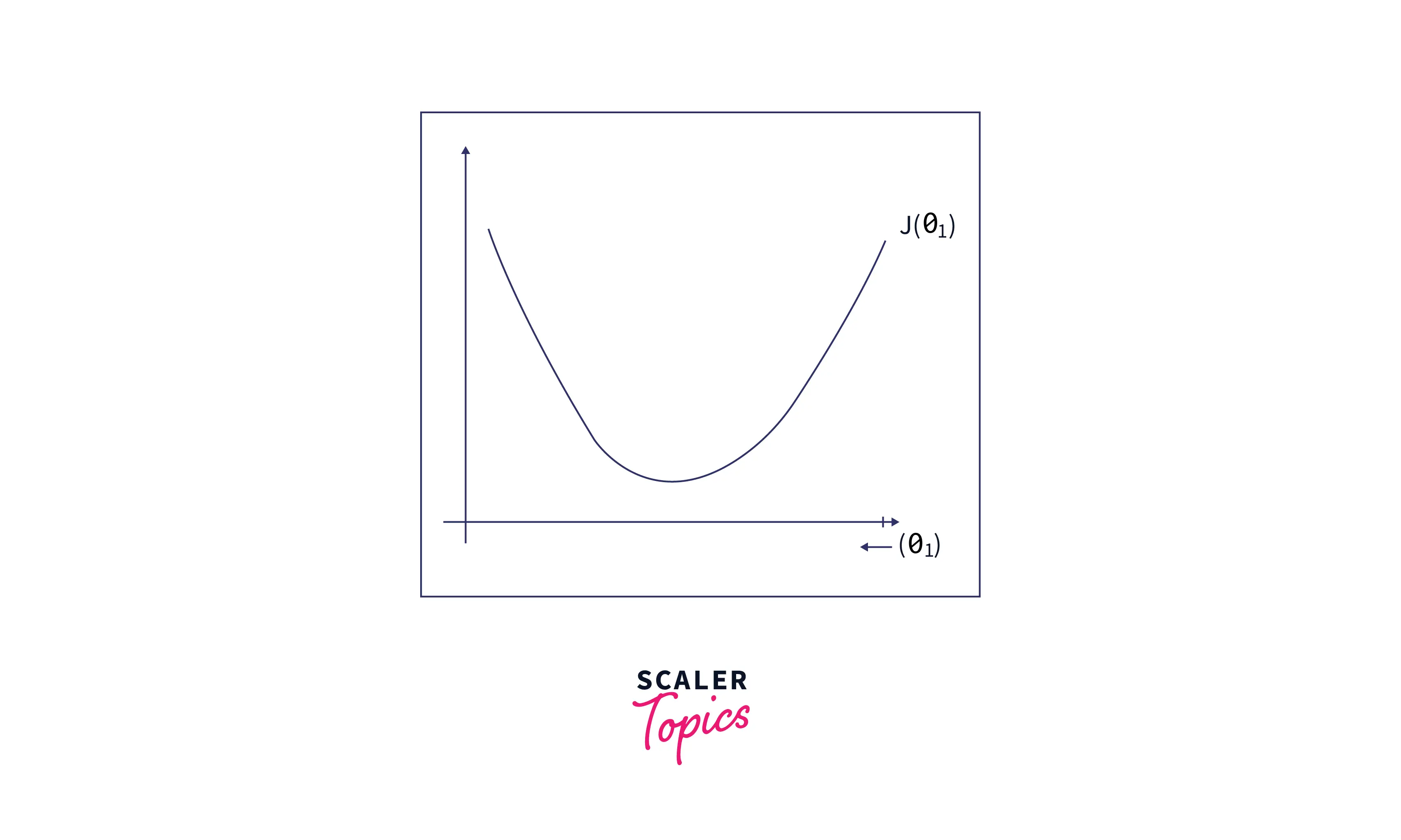
Consider the value of a parameter $θ_1$(theta) that minimizes some arbitrary cost function $J(θ_1)$.

First, let’s plot the cost function $J(θ_1)$ as a function of $θ_1$ as follows:

PS:

For simplicity and easy visualization, we have considered only one parameter. This can be easily extended to multi-dimensions(or multiple parameters)

From the figure above, say that initially, we have chosen some arbitrary value for $θ_1$ and plotted its corresponding cost function value. We can see that the cost function value is quite high.

We can find the apt value for $θ_1$ such that the value of the cost function is minimized as follows:

• Since we have initially assigned an arbitrary value for $θ_1$ and found that the cost function value is high, find the slope at that point.

• If the slope is positive, we can see from the figure below that decreasing the value of $θ_1$ will decrease the cost function value. Hence, go on to decrease the value of $θ_1$ by some small amount.

  

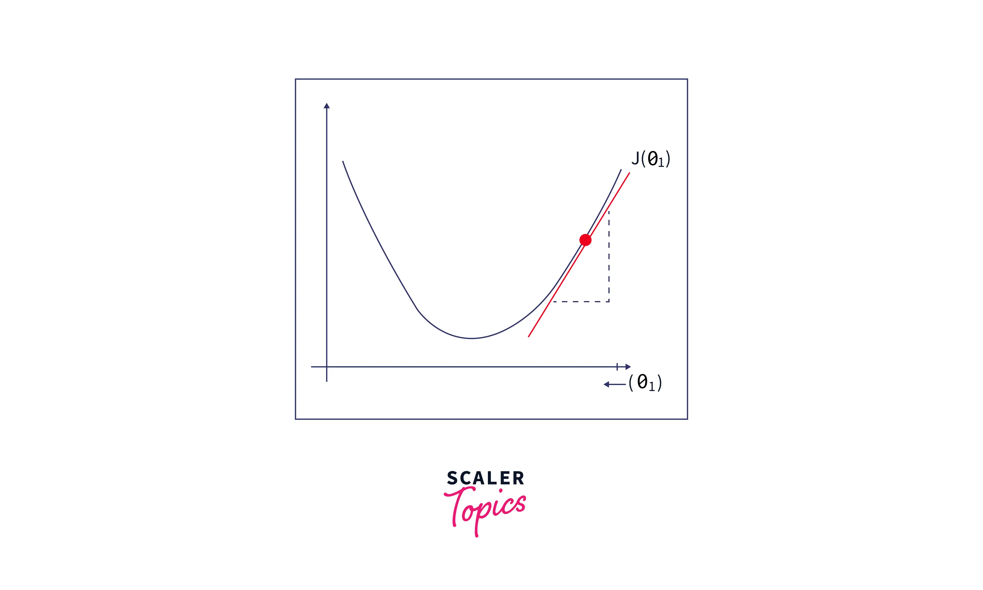
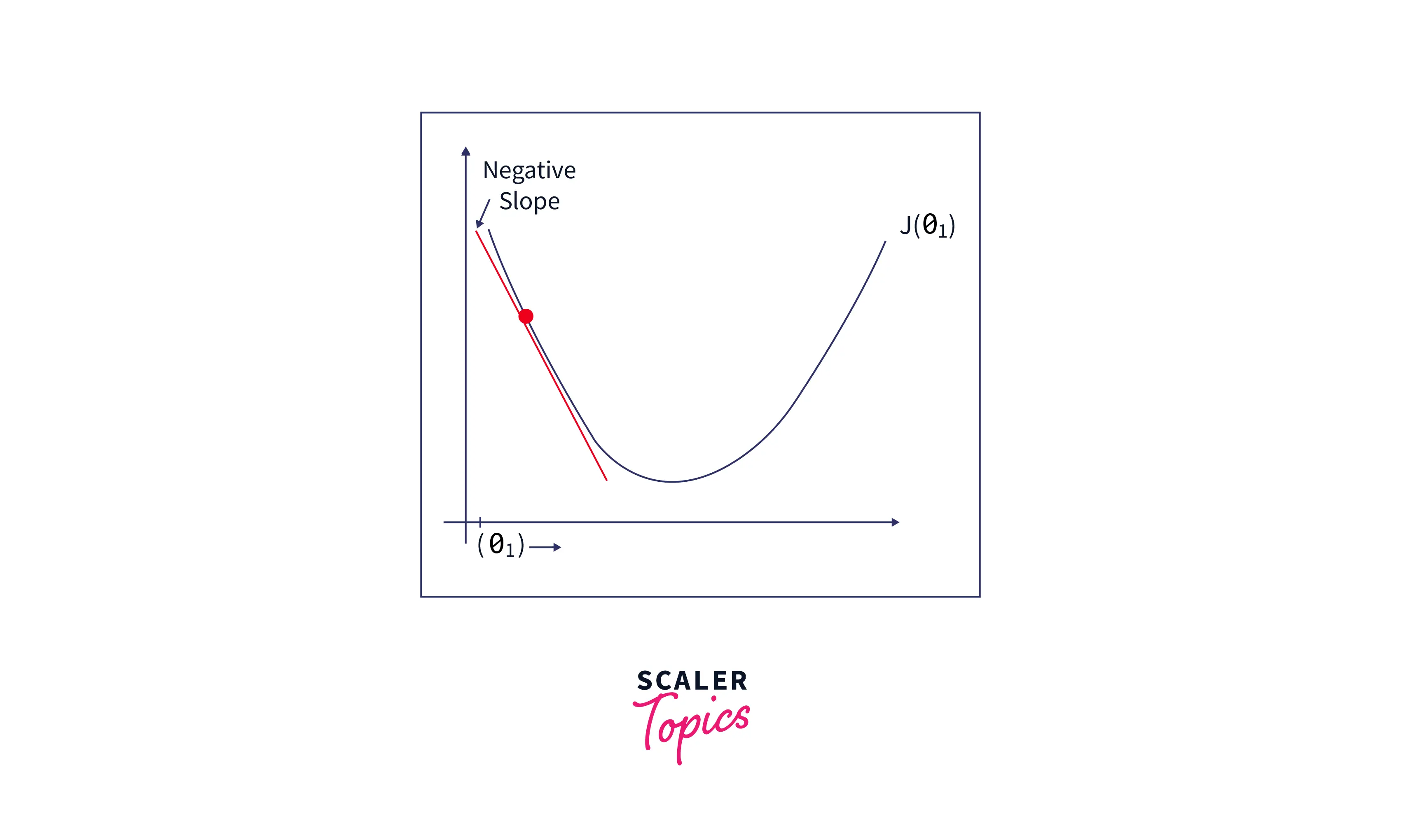
• If the slope is negative, we can see from the figure below that increasing the value of $θ1$ will decrease the cost function value. Hence, go on to increase the value of $θ1$ by some small amount.

  

Let's summarize the above gradient descent concept to a generalized formula:

Here, $\alpha$ designates the learning rate(i.e., how big the gradient descent step should be). Most often, $\alpha$ takes values like 0.01, 0.001, 0.0001, and so on.

$\theta_1:=\theta_1-\alpha \frac{\partial}{\partial \theta_1} J\left(\theta_1\right)$

The above formula is for a single parameter of interest. For two parameters, the value of, say $\theta_1$ and $\theta_2$ can be found as follows:

repeat until convergence

simultaneously update $j=0$ and $j=1$

As we can see, first, you arbitrarily choose the values for $θ_1$ and $θ_2$. You then find the slope of the function at this point and update the value of and as in the formula and do the same until the value decreases/increases very little (This is because as the parameters approach their optimal value(local/global minima), they take very small steps. Hence, the phrase "repeat until convergence").

By following the above method, we can find the required number of parameter values that minimizes the cost function. This, in turn, will help us to find the best values for the weights and biases and make good predictions with minimum loss.

Two Issues of Standard RNNs: Exploding Gradients & Vanishing Gradients

To understand the exploding and vanishing gradients, let us again consider the image below:

The fine-tuning of one hidden layer depends on the next hidden layer and so on. For example, the fine-tuning of the hidden layer $X_{29}$ will depend on the output label $Y_{29}$, the fine-tuning of the hidden layer $X_{28}$ will depend on the hidden layer $X_{29}$, and so on until the weights of the hidden layer $X_{0}$ is reached. As we can see, the tuning of parameters needs to propagate throughout the network from $Y_{29}$ to $X_{0}$.

We can find the problem here. There is a long chain to solve for the apt value of weight or bias as follows:

$\partial \mathrm{E} / \partial \mathrm{W}=\partial \mathrm{E} / \partial \mathrm{y} 3^* \partial \mathrm{y} 3 / \partial \mathrm{h} 3^* \partial \mathrm{h} 3 / \partial \mathrm{y} 2^* \partial \mathrm{y} 2 / \partial \mathrm{h} 1 \ldots$

here,

• $E$ - error function
• $W$ - a weight value
• $Y$ - output
• $h$ - hidden layer weights

If one of the gradients approaches zero, then all will approach zero. The learning will stop very soon. This is called the vanishing gradient problem in rnn architecture.

Sometimes the gradient values will become extremely large, leading to the exploding gradient problem in rnn architecture.

These are the two main problems in the vanilla Recurrent Neural Network Architecture.

Gradient Clipping in RNN

We have the gradient clipping mechanism to overcome the exploding gradient problem in rnn architecture.

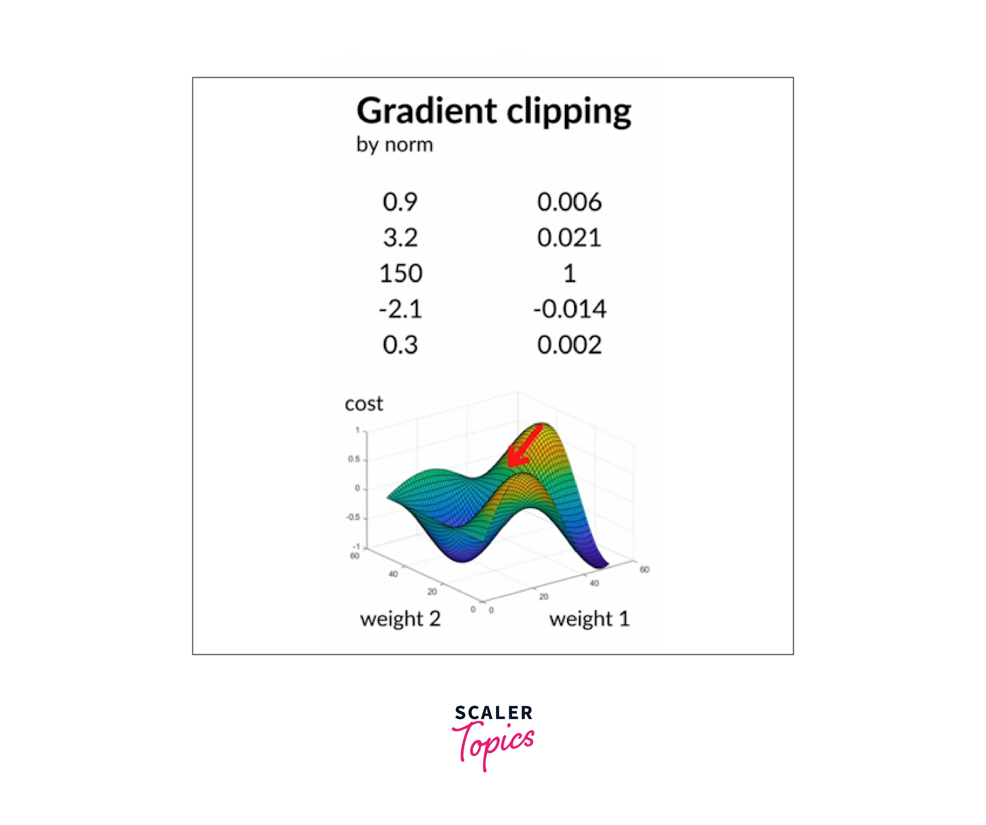
In gradient clipping by norm, the gradient values stay between -1 and +1. The beauty here is that the direction is also maintained such that it moves towards the minimum value of the cost function. This is how gradient clipping by norm overcomes the exploding gradient problem in rnn architecture.

RNN and Long Short-Term Memory (LSTM)

RNNs suffer from another major problem. As the sequence gets longer and longer, the initial information gets forgotten. We can see this in the image below.

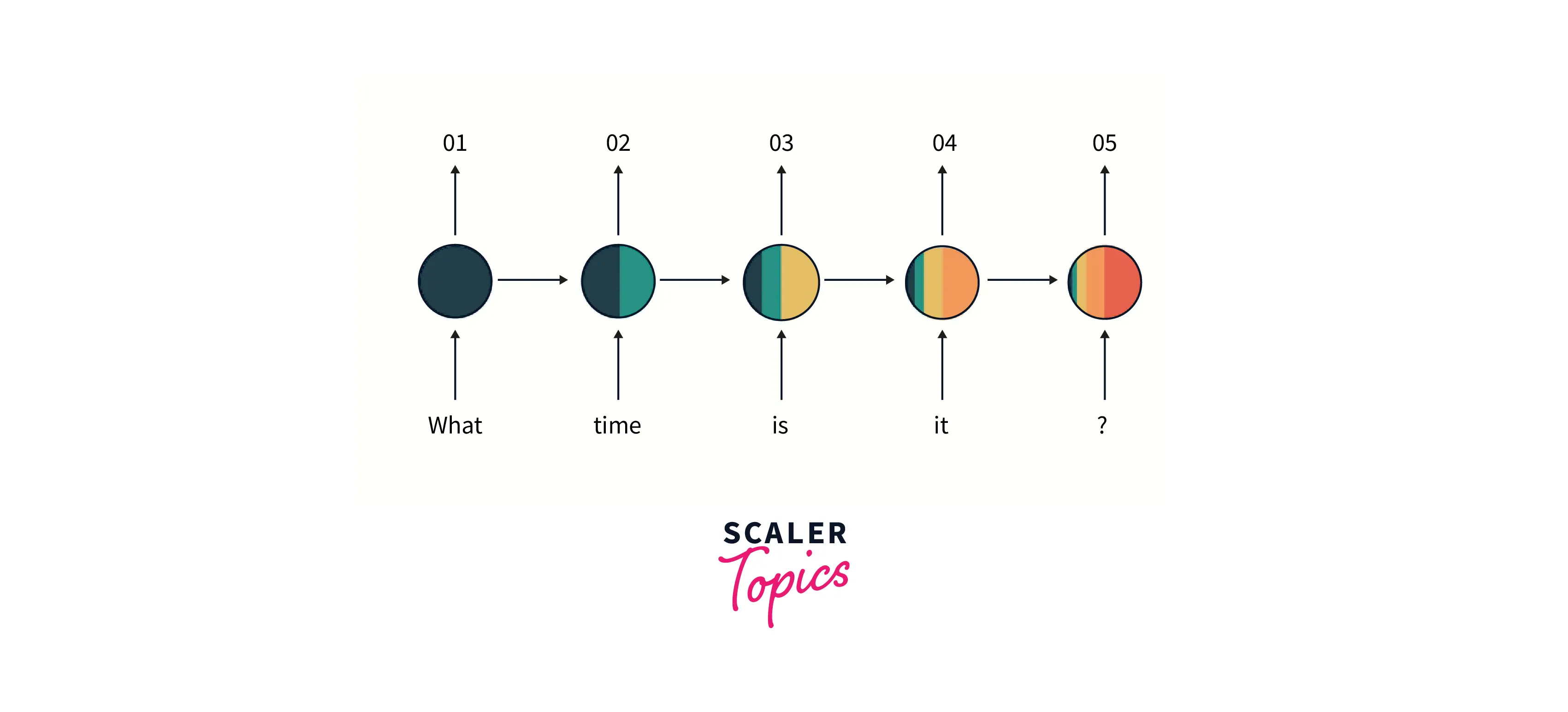
As we go further down the sequence, as indicated by the colors, The knowledge of initial information diminishes.

To overcome this, there are modified versions of the recurrent neural network, such as Long-Short Term Memory(LSTM). LSTM transfers important information further down the network while leaving unnecessary information behind.

Other RNN Architectures

There are two modified architectures of RNN, namely LSTM and GRU(Gated Recurrent Unit). They help in alleviating the above problem of memory.

The overview of the architectures is as follows:

LSTM Cell Architecture(Hidden Layer):

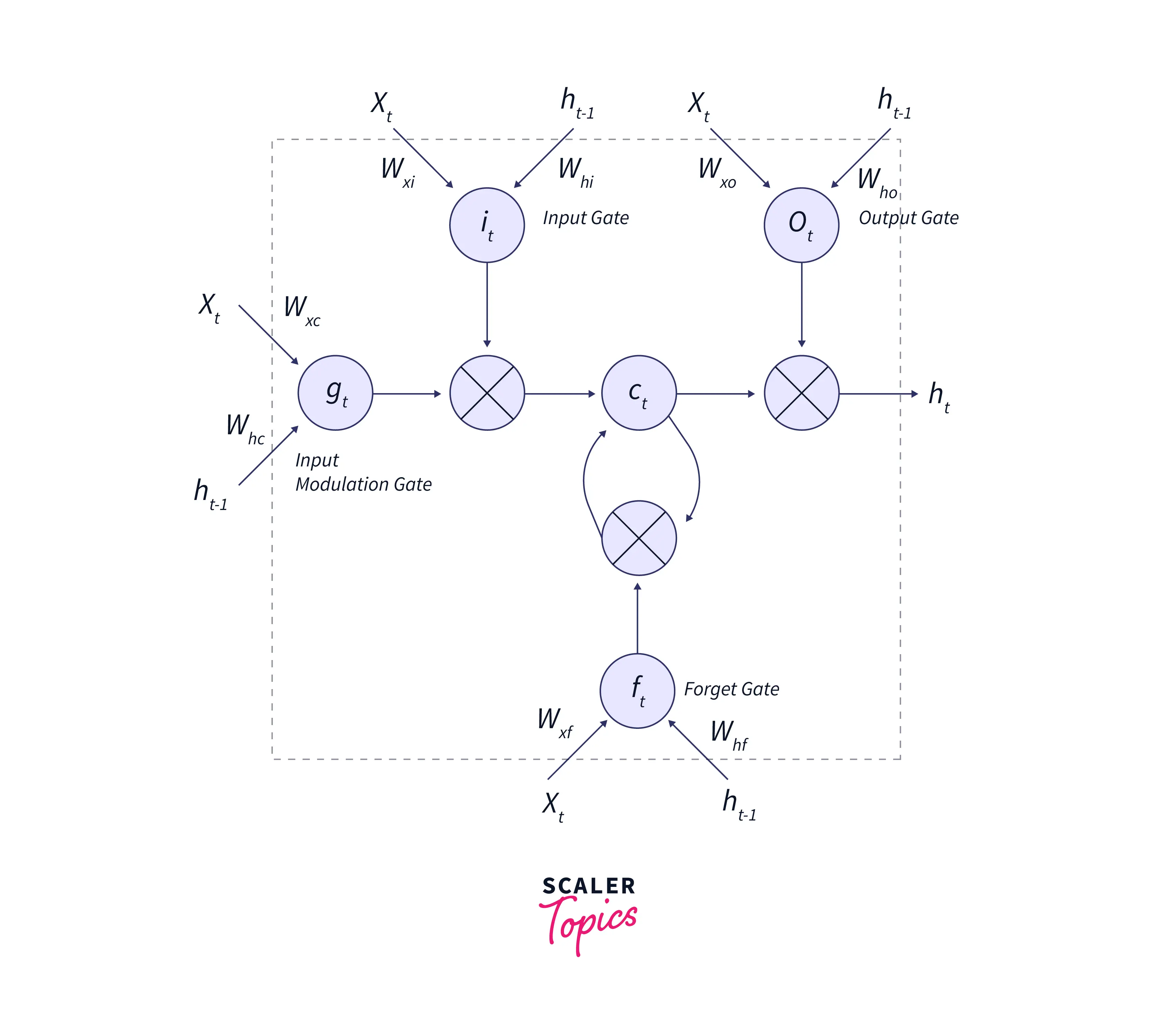
• Forget gate: Gets rid of information that needs to be more important.
• Input gate: Decides what information must be added and tracked from the current timestep.
• Output gate: It influences information to be passed to the next hidden state.

An LSTM cell takes the hidden layer of the previous timestep, current input, and the previous cell state as its input.

GRU Cell Architecture(Hidden Layer):

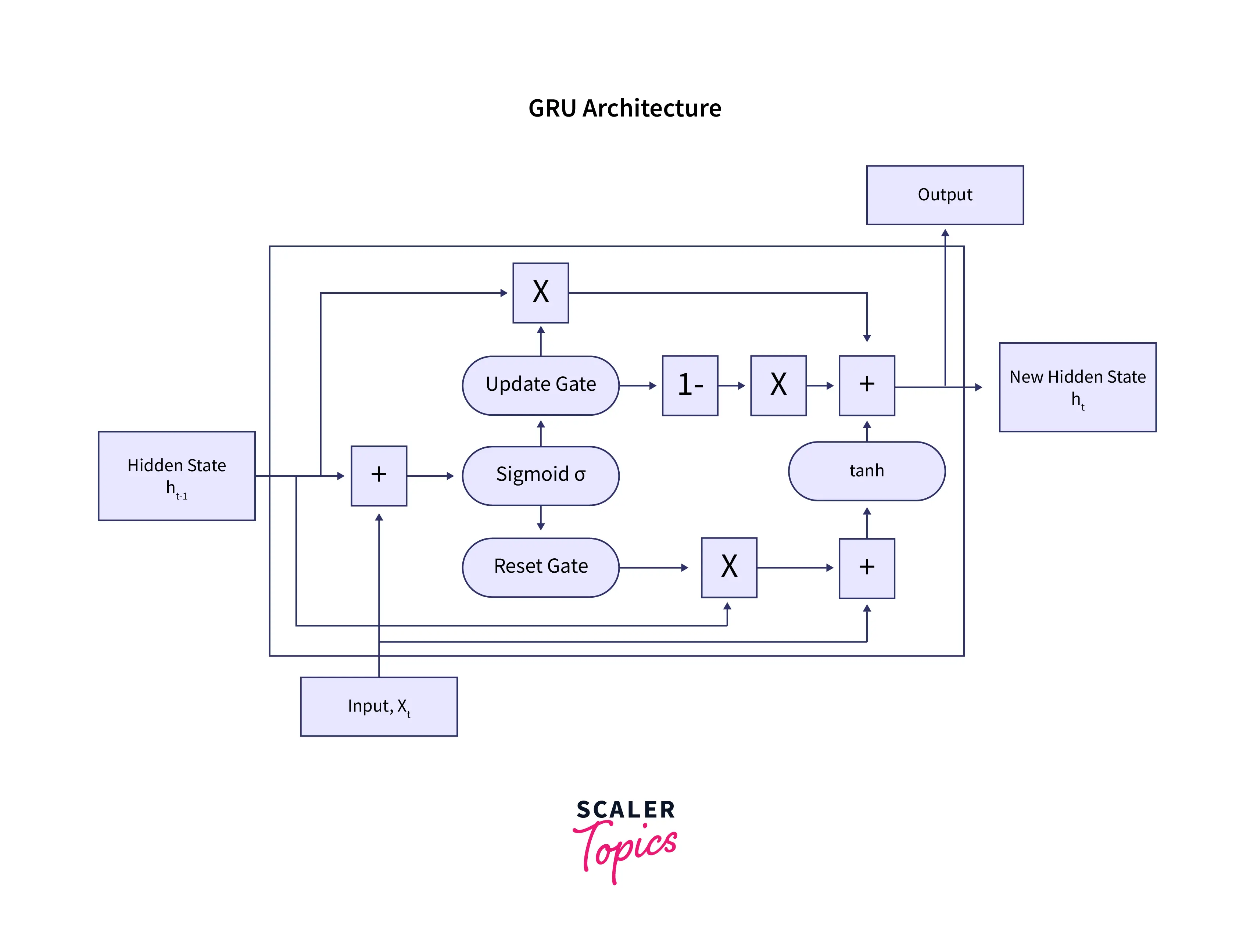
• Update gate: used to pass the important information further down the network.
• Reset gate: Gets rid of information that is not important.

A GRU cell takes the hidden layer of the previous timestep and current input as input.