Sort, Filter, and Transpose in Excel

Pre-requisistes

You should have a fundamental understanding of Excel's interface and terminology before using its sorting, filtering, and transposition tools. It is also helpful to have some experience working with data in Excel, such as building and formatting tables, entering data, and utilizing basic calculations and functions.

Introduction

Microsoft Excel is a powerful tool for organizing and analyzing data. You may sort, filter, and transpose in Excel using a number of its capabilities to make it more helpful and accessible. You may easily group information based on specific criteria, such as alphabetical order or numerical value, by sorting the data. You can focus on particular areas of a table by focusing on the information you have filtered down to show you. You can rearrange tables to make them simpler to read and use by transposing data.

Learning how to sort, how filter and transpose in Excel will help you work more effectively and efficiently, regardless of whether you are a business analyst, data scientist, or simply someone who works with data regularly.

How to Transpose in Excel?

TRANSPOSE in Excel involves changing the direction of the data from rows to columns or vice versa. This can be helpful if you need to run computations on a new set of data or reorganize your data. With Excel, you can transpose in Excel by several different methods, such as by using the Paste Special Transpose function, the TRANSPOSE function, or the Power Query tool. We will look at them one by one.

Paste Special Transpose

Using Paste Special Transpose in Excel is a quick and easy way to transpose data in a table or range of cells. Here are the steps to use this feature:

• Select the range of cells that you want to transpose.

• Right-click on the selected cells and choose "Copy" or press the "Ctrl + C" shortcut key.

• Right-click on a blank cell where you want to paste the transposed data and choose "Paste Special" from the menu.

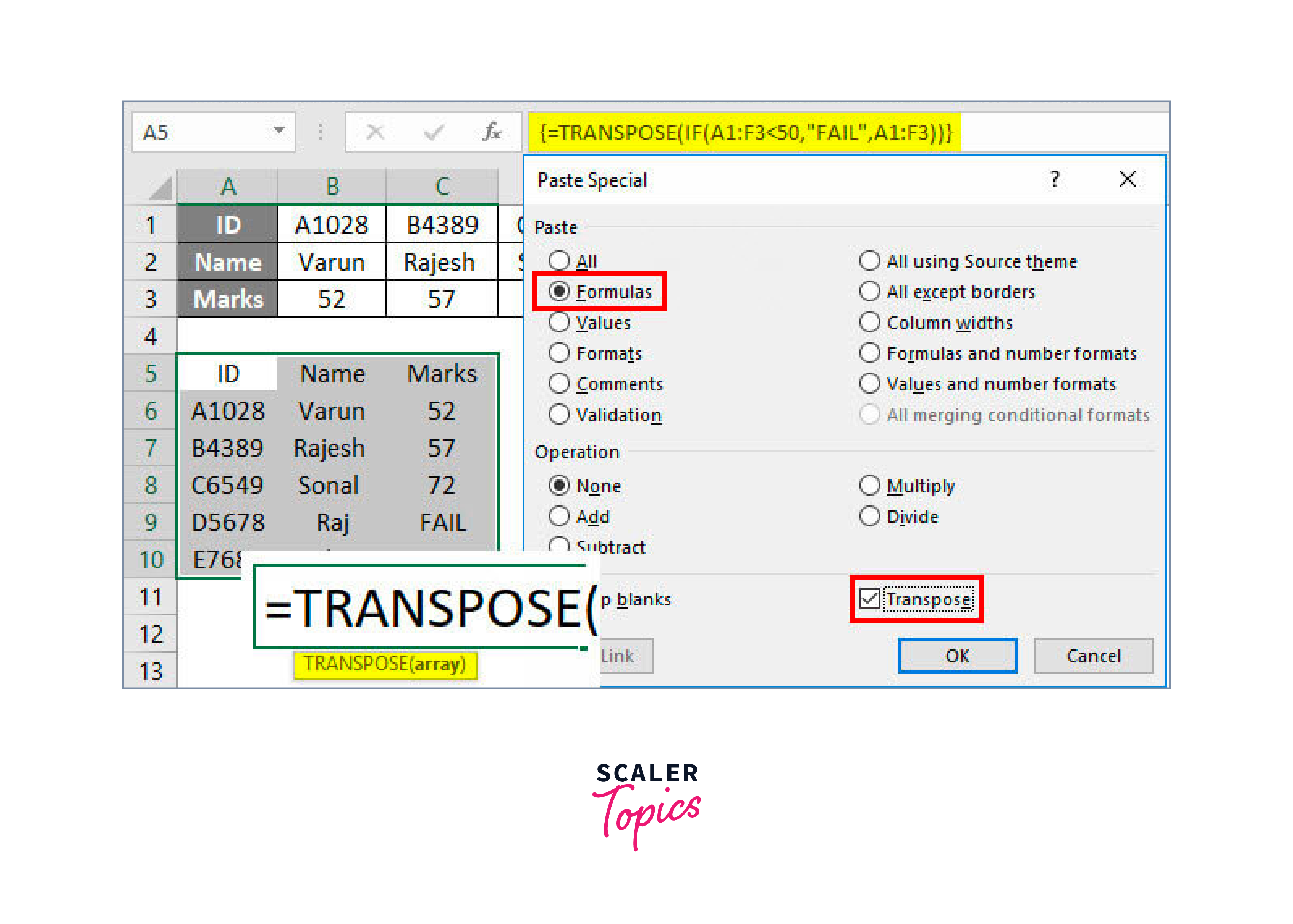
• In the Paste Special dialog box, check the "Transpose" option and click "OK".

  

• The data will be pasted and transposed into the new location.

It's important to note that when using Paste Special Transpose in Excel, the original data is not deleted or moved. Rather, a new transposed version of the data is created in the new location. This means that you can still access and work with the original data as needed.

TRANSPOSE Excel Function

In addition to using Paste Special Transpose in Excel, you can also use the TRANSPOSE Excel function to transpose data. Here are the steps to use this feature:

• Select the range of cells that you want to transpose.
• Click on a blank cell where you want to paste the transposed data.
• Type the following formula into the formula bar: TRANSPOSE(range), where "range" is the range of cells that you want to transpose in Excel.
• Press "Ctrl + Shift + Enter" to enter the formula as an array formula.
• This is necessary because the TRANSPOSE function returns an array of values rather than a single value.
• The data will be pasted and transposed into the new location.

Using Power Query Tool

Power Query is a powerful data transformation and cleaning tool in Excel that can be used to extract, transform, and load data from a variety of sources. Here are the steps to use Power Query to transpose data in Excel:

• Select the range of cells that you want to transpose in Excel.

• Go to the Data tab and select "From Table/Range" under the "Get & Transform Data" section.

• In the Power Query Editor, select the "Transform" tab.

• Click on the "Transpose" button.

• Click "Close & Load" in the "Home" tab of the ribbon to close the Power Query Editor and load the transposed data into a new worksheet.

  Power Query offers much more flexibility and control over the data transformation process than the Paste Special Transpose or TRANSPOSE functions, but it can be slightly more difficult to use. Power Query is a useful tool for everyone who deals with data in Excel because it can also be used to carry out a wide range of additional data transformations and cleaning activities.

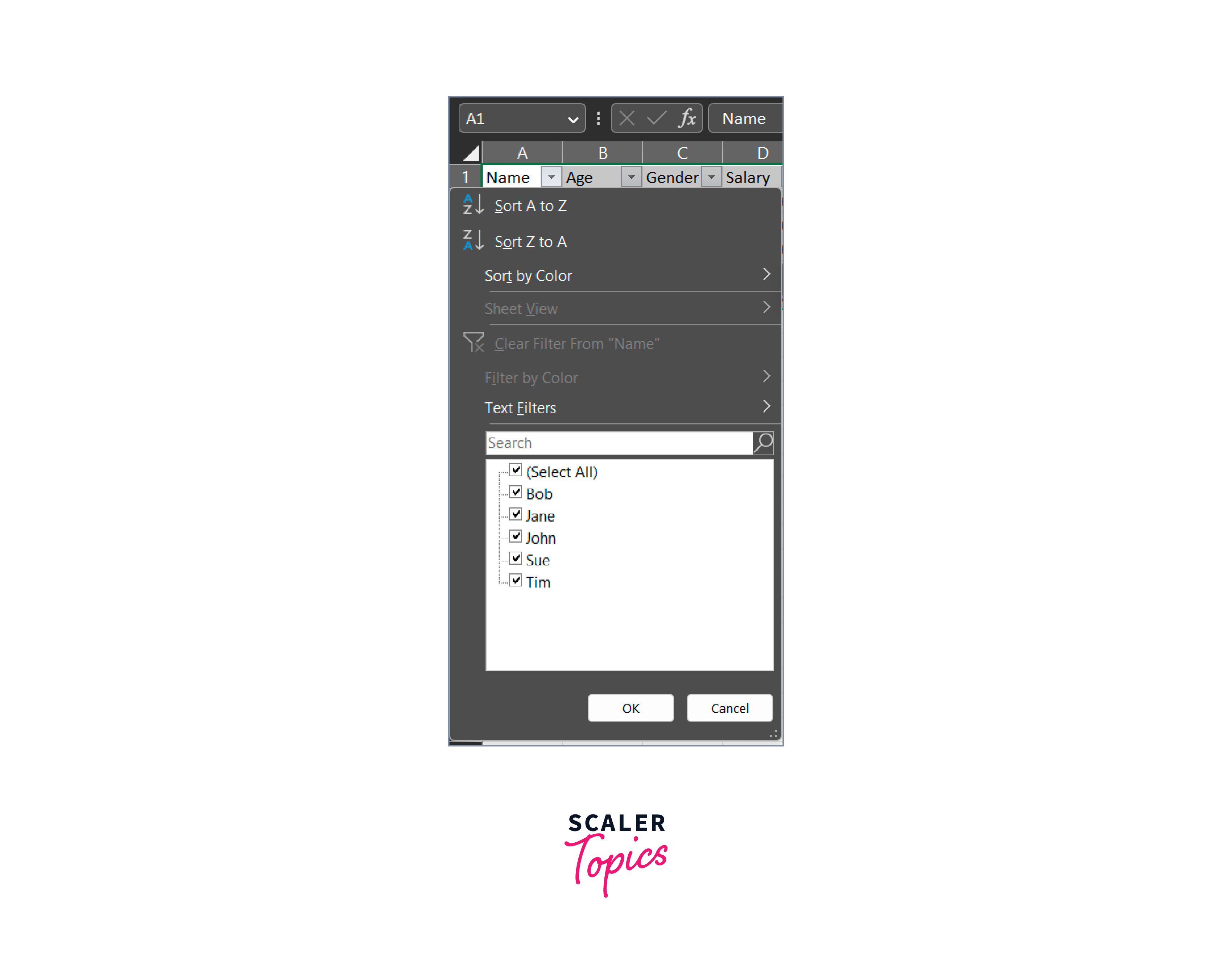
How to Filter in Excel?

In Excel, filtering is the process of showing only particular rows or columns of data based on predetermined standards or conditions. It enables you to keep the remainder of the data accessible while hiding the rows or columns that don't match your filtering criteria.

When you have a large dataset and want to concentrate on a certain subset of the data that satisfies certain criteria, filtering might be helpful. For instance, you could just want to view the sales information for a certain product or a certain period. You may quickly and easily display only the rows that satisfy your criteria while concealing the rest of the data by filtering the data. Thus it is important to learn how to filter in Excel. There are three ways to filter in Excel.

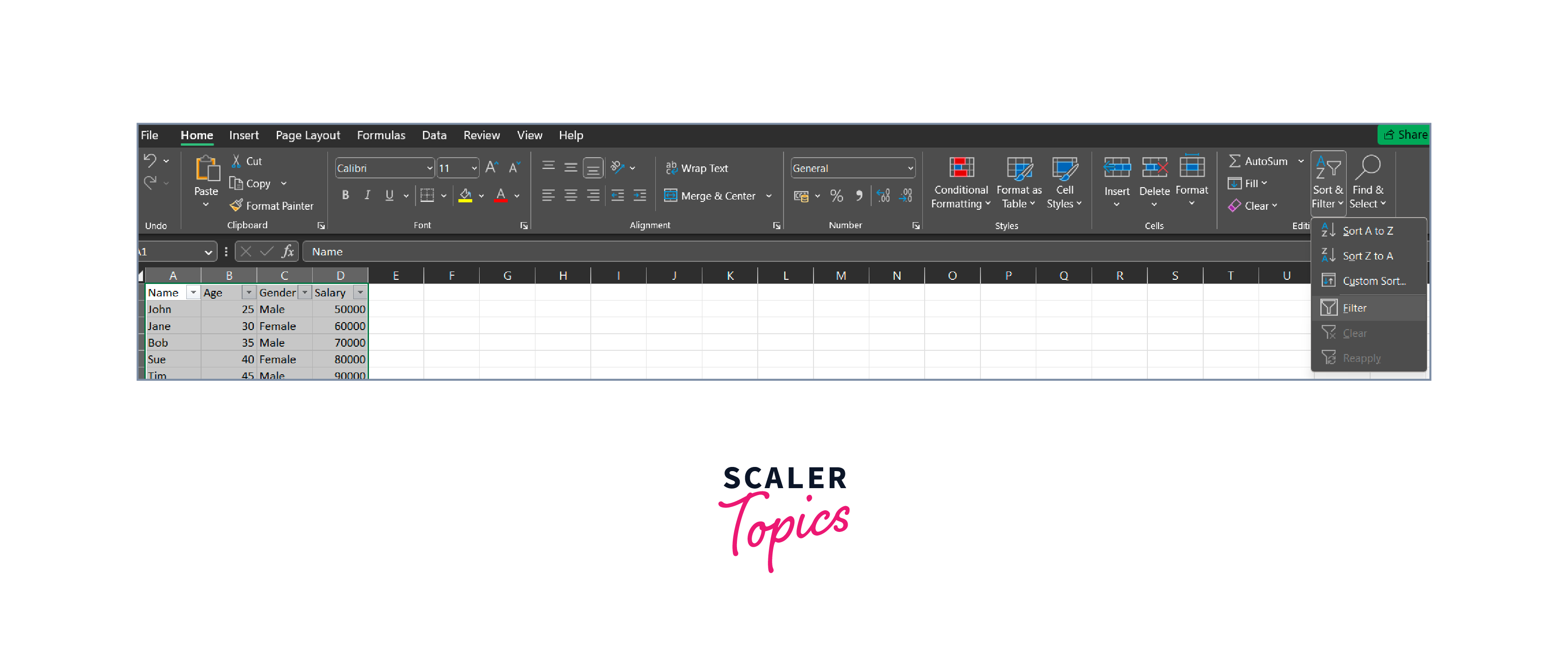
With Filter Option Under the Home Tab

To filter data use the Filter option under the Home tab:

• Select the data you want to filter.
• Click on the "Filter" button under the Home tab.
• Use the filter dropdowns to select the data you want to display.

With Filter Option Under the Data Tab

To filter data use the Filter option under the Data tab:

• Select the data you want to filter.
• Click on the "Filter" button under the Data tab.
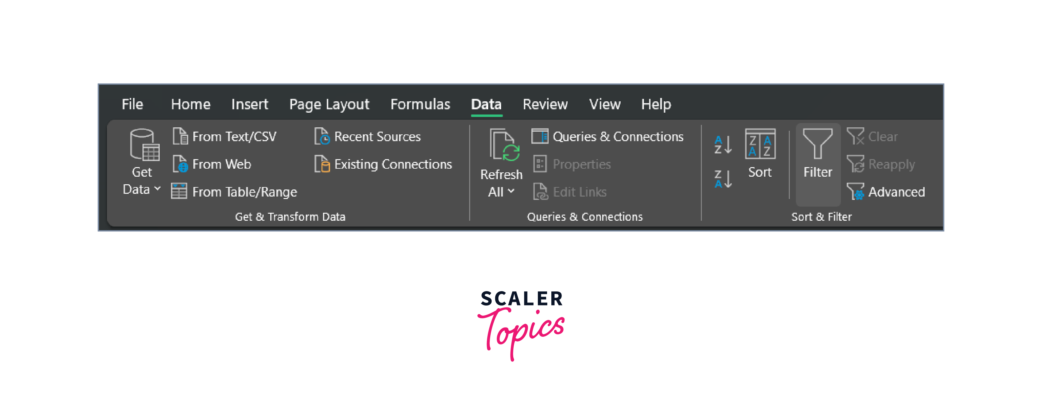
• Use the filter dropdowns to select the data you want to display.

With the Shortcut Key

To filter data using the shortcut key:

• Select the data you want to filter.
• Press "Ctrl+Shift+L".
• Use the filter dropdowns to select the data you want to display.

SORT Function

The Excel SORT function is a powerful tool that allows you to sort data in ascending or descending order based on one or more columns. It can be used to quickly and easily reorder rows or columns of data based on specific criteria, making it easier to analyze and understand large datasets.

Syntax

Here's the syntax for the Excel SORT function:

Parameters

• array: Required The range of cells to sort.
• sort_index: Optional The column or row number to sort by. The default is 1.
• sort_order: Optional The order to sort by. "Ascending" or "Descending". The default is "Ascending".
• by_col: Optional A logical value that indicates whether to sort by columns or rows. The default is TRUE (columns).

Return

The Excel SORT function returns a sorted array or table.

Example

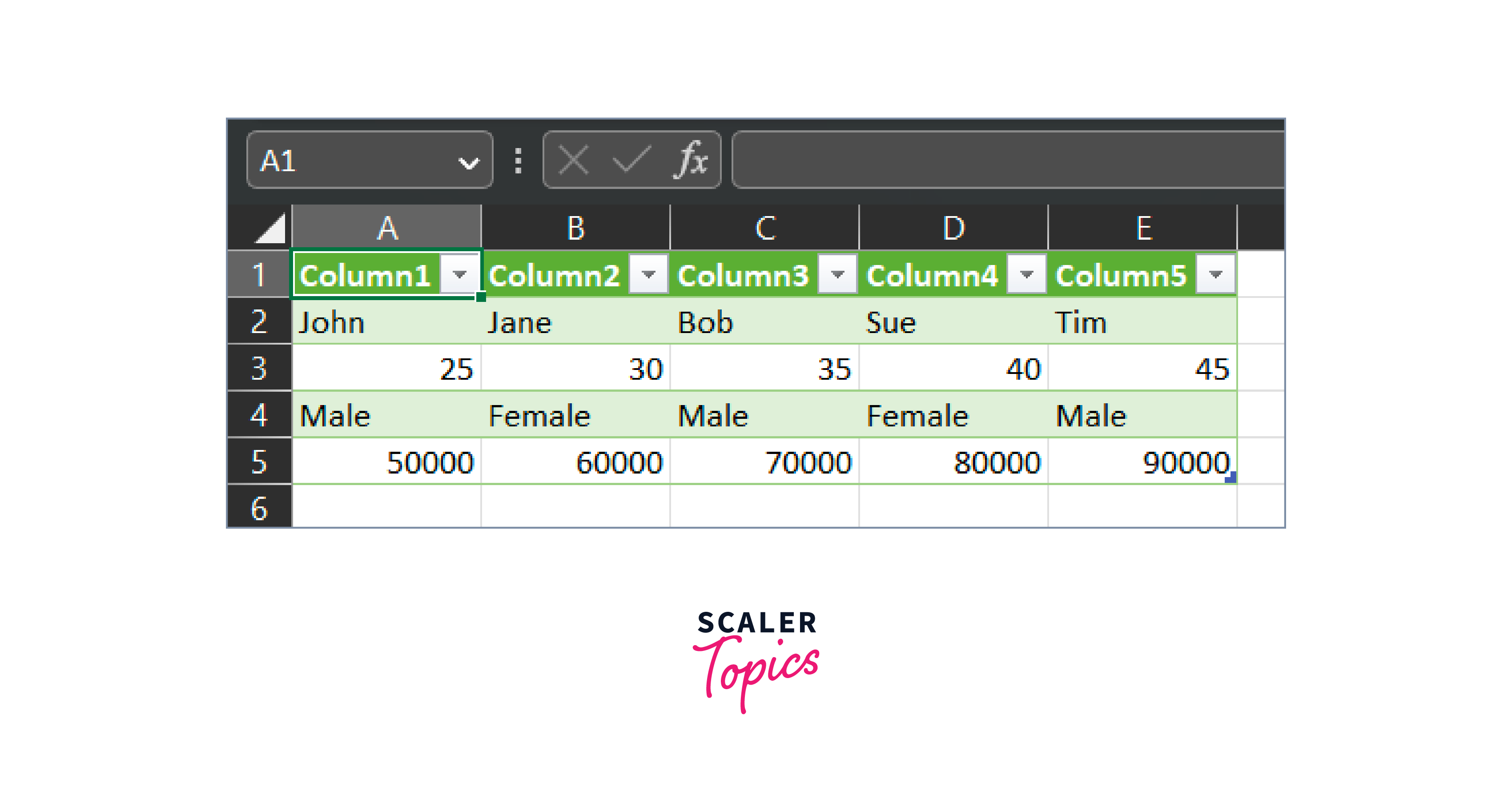
Let's say you have a table of data in cells A1:D5, with the following values:

To sort this table by age in descending order, you would use the following formula:

Here the value in sort_index is 2 so it sorts the data based on Age. The value in sort_order can be 1 or -1 to sort it in ascending order and descending order respectively. Here it sorts the table in descending order.

This would return the following sorted table:

Usage

• The Excel SORT function can be used in a variety of situations, including arranging data for analysis, sorting data in tables, and producing reports.
• When you want to arrange data in a precise order, sorting the data is frequently helpful. Sorting the data might make it easier to read and evaluate, for instance, if you have a list of student grades and you want to organize them in order from highest to lowest.
• When you need to use the data for computations or analysis, sorting it can be useful. Sorting the data can make it simpler to execute calculations, for instance, if you need to perform calculations on a certain subset of a huge dataset.

How to Search in Excel?

Microsoft Excel is a powerful tool for managing and organizing data. However, when working with large sets of data, finding specific information can be time-consuming and frustrating. Fortunately, Excel provides several methods for searching data, including the Find and Replace function, using filters, sorting data, and using the OFFSET function. Here are a few ways to search in Excel.

1. Find and Replace Function

• The Find and Replace function is a powerful tool that allows users to search for specific data in a worksheet and replace it with new information if necessary.
• To use this function, follow these steps:
  • Press Ctrl+F or go to the Home tab and click on the Find & Select button, then click on "Find".
  • In the "Find and Replace" dialog box, type in the search term and click on the "Find Next" button.
  • If the search term is found, it will be highlighted in the worksheet.
  • To replace the search term with new information, click on the "Replace" button.

2. Using Filters

• Filtering data in Excel allows you to display only the rows that meet specific criteria.
• By filtering your data, you can easily locate and identify specific data points

3. Sorting Data

• Sorting data in Excel allows you to arrange the rows or columns in a specific order based on selected criteria.
• By sorting your data, you can easily locate and identify specific data points.

4. Using the OFFSET Function

• The OFFSET function is a powerful tool that allows users to search for data by offsetting from a starting point.
• To use this function, follow these steps:
  • In an empty cell, type in the formula "=OFFSET(starting cell, rows to offset, columns to offset)".
  • Replace "starting cell" with the cell you want to start from, "rows to offset" with the number of rows you want to offset, and "columns to offset" with the number of columns you want to offset.
  • Press Enter to display the search result.

5. Transposing data

• Transposing data in Excel allows you to switch the orientation of your data from rows to columns, or vice versa.
• By transposing your data, you can easily locate and identify specific data points.

Hence, there are several methods available to search for data in Excel. The Find and Replace function, filtering, sorting data, transposing, and using the OFFSET function are all powerful tools that can help users quickly find the information they need. By utilizing these methods, users can save time and work more efficiently in Excel.

For example, if you are looking for the highest or lowest values in a column, you can sort the column in descending or ascending order, respectively. If you are looking for data points that meet specific criteria, you can use the filtering tool to display only the rows that meet those criteria. If you need to re-orient your data to search for specific values, you can use the transpose tool in Excel to switch the orientation of your data.

OFFSET Function in Excel

The OFFSET function is used to return a reference to a range that is a specified number of rows and columns away from a starting cell or range.

Syntax

Parameters

• reference: Required The starting cell or range of cells.
• rows: Required The number of rows to move away from the starting cell or range. Positive values move down, while negative values move up.
• cols: Required The number of columns to move away from the starting cell or range. Positive values move right, while negative values move left.
• height: Optional The height of the range to return. The default is the same height as the reference.
• width: Optional The width of the range to return. The default is the same width as the reference.

Example

This formula will return a reference to a range that is two rows down and one column right from cell A2. The range will be two rows high and two columns wide.

Usage

• The OFFSET function is often helpful when you need to return a reference to a specific cell or range of cells. For example, if you have a large dataset but only need to work with a specific range of cells, using the OFFSET function can make it easier to work with the data.
• The OFFSET function can also be helpful when you need to perform calculations or analysis on specific data. For example, if you have a large dataset and you need to perform calculations on a specific subset of the data, using the OFFSET function can make it easier to perform the calculations.