Strassen's Matrix Multiplication

Problem Statment

Consider two matrices X and Y each of the size N*N. We want to calculate the resultant matrix Z which is formed by multiplying the given two matrices i.e, X and Y.

Example

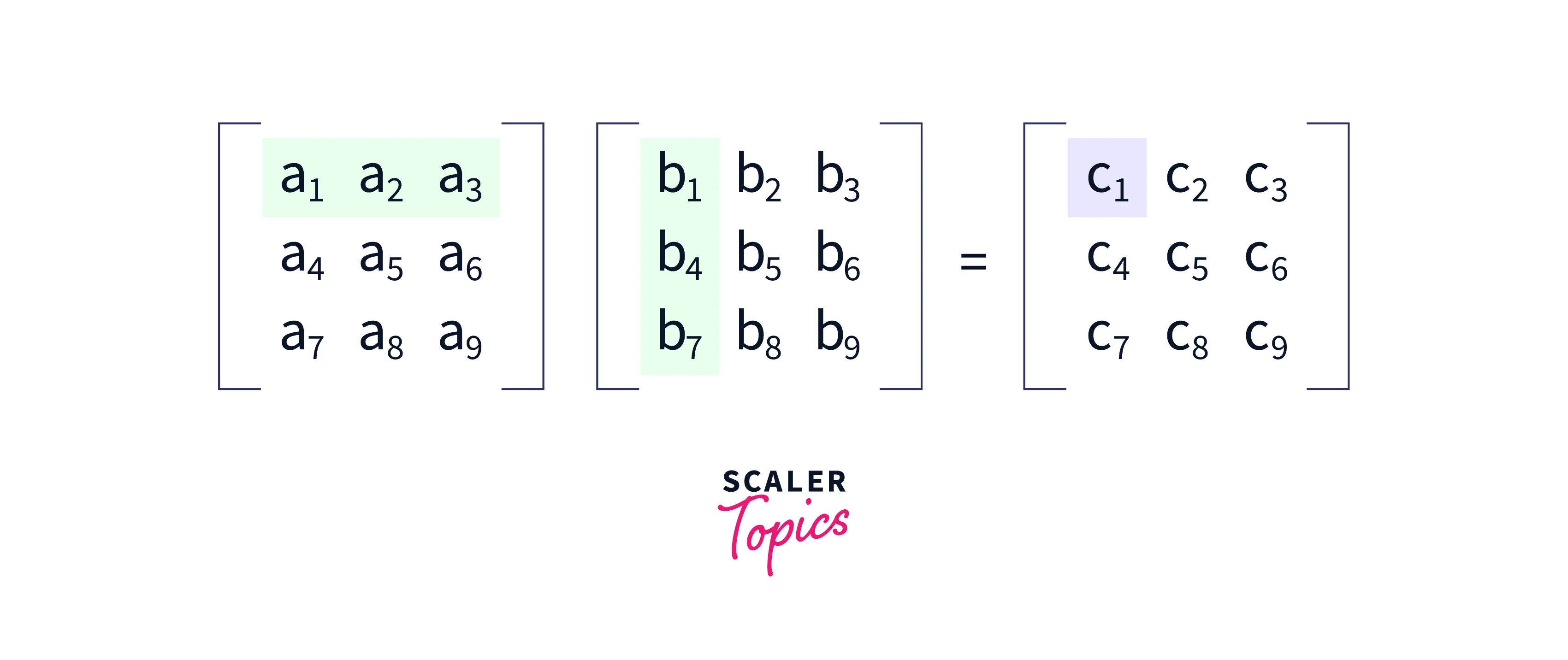
Let's consider the below matrices for multiplication. Matrix A has a size N*M and matrix B has a size A*B. Given two matrices are multiplied only when the number of columns in the first matrix is equal to the number of rows in the second matrix. Therefore, we can say that matrix multiplication is possible only when M==A. The given two matrices are: Matrix A of the size: 3 × 3

The second matrix B of the size : 3 × 3

From the given matrices, since the condition is satisfied it can be multiplied as :

Therefore the result of the multiplication is :

Explanation

We know that,

Below image clearly how matrices are multiplied:

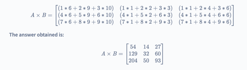
Therefore, the matrix multiplication of given matrices A and B is:

The answer obtained is:

Approach 1: Naive Method

As we have observed in the previous example discussed that the row values are multiplied with each column value and are added to the present value at that cell. By following the below algorithm, a naive method we can obtain the matrix multiplication of given two matrices.

Algorithm: Below is the algorithm for Matrix Multiplication using a naive method:

• Firstly, the number of rows in the second matrix should be the same as the number of columns in the first matrix.
• The size of matrix 1 is N × M and the size of the second matrix is M × P .
• Now, initialize the resultant matrix of size as the number of rows of the first matrix and the number of columns as the second matrix. Therefore the size of the resultant matrix is considered to be as N × P.
• For obtaining the values in the resultant matrix three nested loops are used:
  • First nested loop represents the row number in the matrix. This loop starts at 0 and ends at N.
  • Second nested loop represents the column number in the matrix. This loop starts at 0 and ends at M.
  • And the last nested loop is used for adding the values when each row element is multiplied with all elements in the column respectively.
• Finally, matrix multiplication is done and the values are stored in the resultant matrix.

Implementation

Below is the implementation of this naive approach for matrix multiplication in C++, Python, and Java.

C++ Implementation of Multiplication of Matrices Using the Naive Method:

Output:

Python Implementation of Multiplication of Matrices Using the Naive Method:

Output:

Java Implementation of Multiplication of Matrices Using the Naive Method:

Output:

Explanation:

The given two matrices are multiplied and the result has been printed as the output.

Complexity Analysis

Time Complexity: O(N^3), where the given matrices are square matrices of size N*N each.

• For multiplying every column with every element in the row from the given matrices uses two loops, and adding up the values takes another loop. Therefore the overall time complexity turns out to be O(N^3^).

Space Complexity: O(N^2), where the given matrices are square matrices of size N*N each.

• The matrix of size N*N has been used to store the result when the two matrices are multiplied.

Approach 2: Using Strassen’s Matrix Multiplication

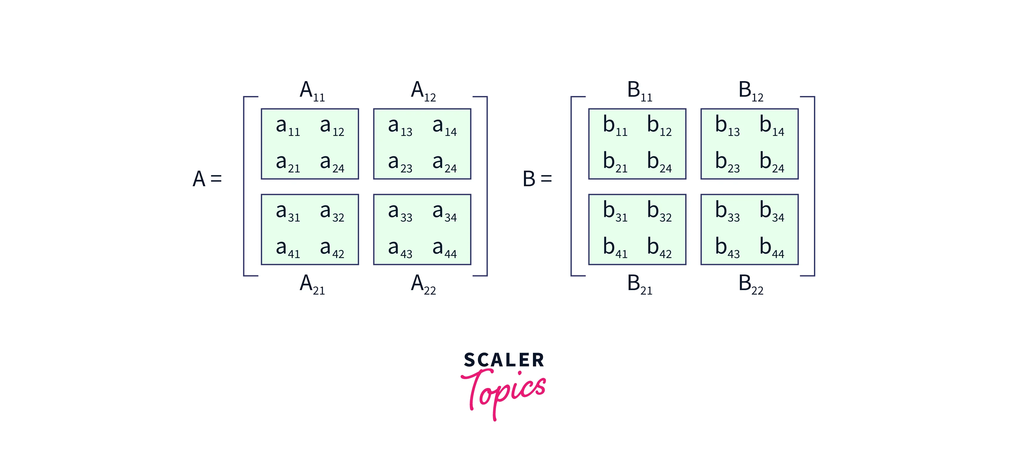
• To optimize the matrix multiplication Strassen's matrix multiplication algorithm can be used. It reduces the time complexity for matrix multiplication. Strassen’s Matrix multiplication can be performed only on square matrices where N is a power of 2. And also the order of both of the matrices is N × N.

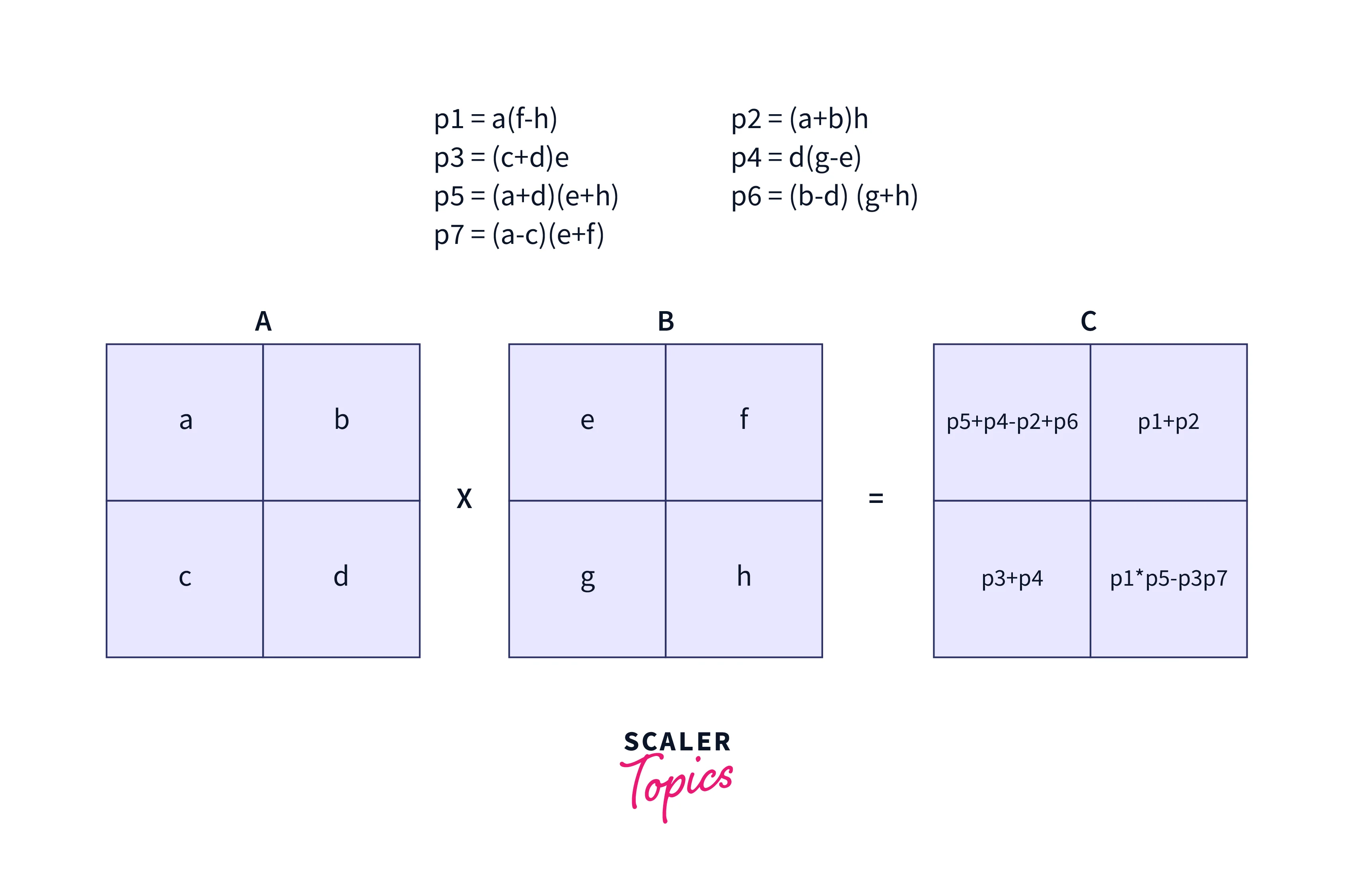
• The main idea is to use the divide and conquer technique in this algorithm. We need to divide matrix A and matrix B into 8 submatrices and then recursively compute the submatrices of the result.

• In the above approach we are doing $N^3$ multiplications and $N^2$ additions are performed. Therefore the overall time complexity is $O(N^3)$. We need to divide the given A and B matrices each of order $N_2 × N_2$.

• This can be clearly explained in the below image:

• For each multiplication of size $N_2 × N_2$, follow the below recursive function as shown in the figure:

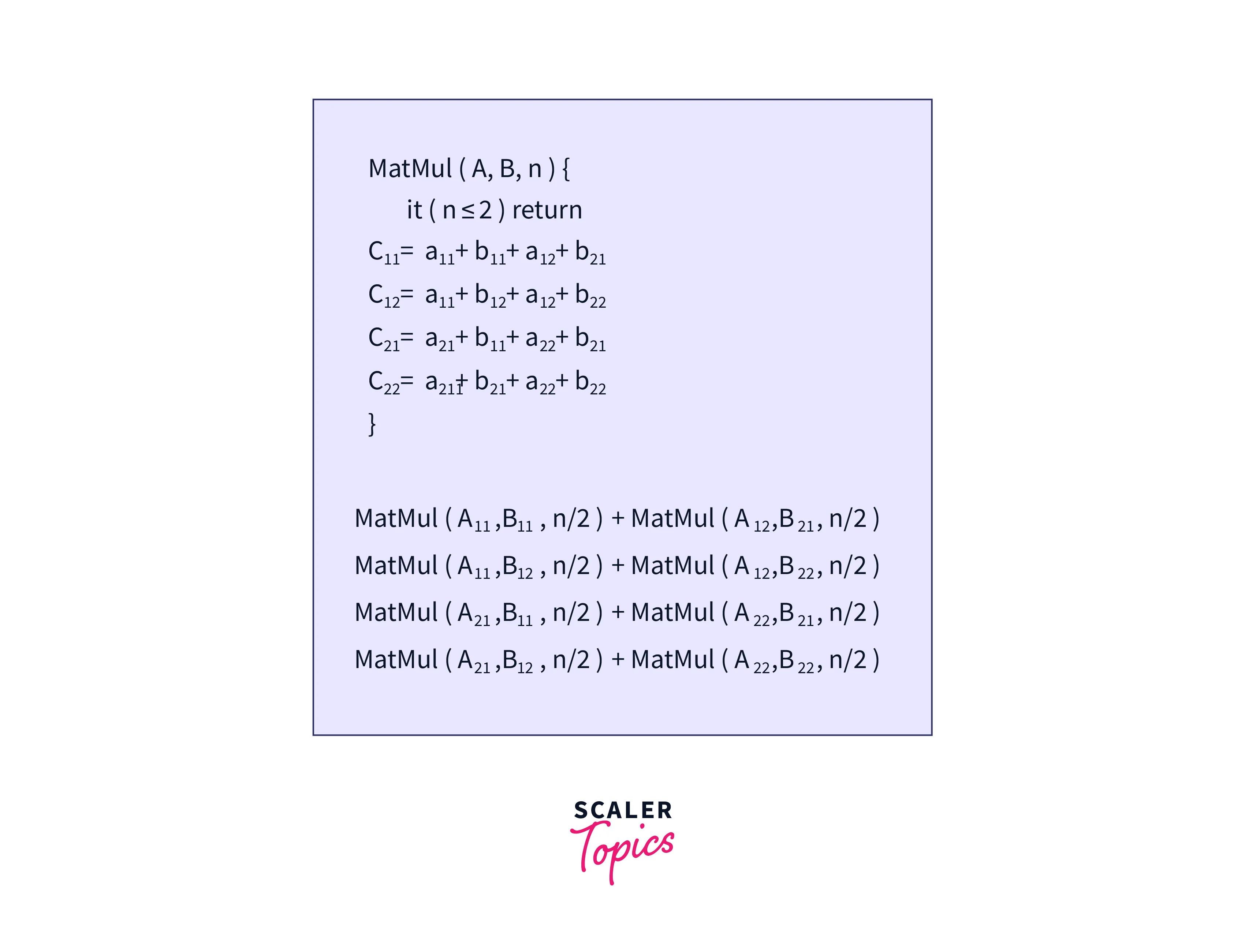
• Where the resultant matrix is C and can be obtained in the following way. Now we need to store the result as follows:

  • $C_{11}= A_{11} *B_{11} + A_{12} *B_{21}$
  • $C_{12}= A_{11} *B_{12} + A_{12} *B_{22}$
  • $C_{21}= A_{21} *B_{11} + A_{22} *B_{21}$
  • $C_{22}= A_{21} *B_{12} + A_{22} *B_{22}$

• The recurrence relation obtained is: $T(N) = 8 T(N_2) + 4 O(N^2)$

• Here O(N^2) term is for matrix addition. Since, addition is performed 4 times during the recursion, Therefore, it is 4 times $O(N^2)$.

• The recurrence relationship can be simplified using the Master's Theorem.

• And the overall time complexity turns out to be $O(N^3)$ which is not better than the naive method which is discussed earlier.

• To optimize it further, we use Strassen’s Matrix Multiplication where we don't need 8 recursive calls, as we can solve them using 7 recursive calls and this requires some manipulation which is achieved using addition and subtraction.

• Strassen’s 7 calls are as follows:

  • $p_{1}= ( A_{11} ) * ( B_{11} - B_{22} )$
  • $p_{2}= ( A_{11} + A_{12} )* ( B_{22} )$
  • $p_{3}= ( A_{21} + A_{22} ) * ( B_{11} )$
  • $p_{4}= ( A_{22} ) * (B_{21} + B_{22})$
  • $p_{5}= ( A_{11} + A_{22} ) * ( B_{11} + B_{22} )$
  • $p_{6}= ( A_{12} - A_{21} ) * ( B_{21} + B_{22} )$
  • $p_{7}= ( A_{11} - A_{21} ) * ( B_{11} + B_{12} )$

Now the resultant matrix can be obtained in the following way:

Therefore Strassen’s Matrix Multiplication algorithm has better time complexity and is considered to be more efficient than the other methods for matrix multiplication.

Algorithm:

1. Divide the given matrix A and matrix B into 4 sub-matrices of size each $N_2 x N_2$ as shown in the above diagram.
2. Now, compute Strassen’s 7 calls recursively.
3. Calculate the submatrices of C.
4. Now, we combine these submatrices into our new resultant matrix C.

Implementation

Below is the implementation of Strassen’s Matrix Multiplication algorithm.

C++ Implementation of Strassen’s Matrix Multiplication Algorithm:

Output:

Python Implementation of Strassen’s Matrix Multiplication Algorithm:

Java Implementation of Strassen’s Matrix Multiplication Algorithm:

Output:

Explanation:

The given two matrices are multiplied and the result has been printed as the output. The condition for Strassen’s Matrix Multiplication algorithm is that the given matrices should be square matrices and of order $N * N$, where N is the power of 2.

Complexity Analysis

Time Complexity: O(N^log(7)), where N * N is the order of square matrices given.

• We just need 7 recurrences Strassen’s Matrix Multiplication algorithm and some addition subtraction has to be performed to manipulate the answer. The recurrence relation obtained is: $T(N) = 7T(N_2) + O(N^2)$
• By solving the above relation, we get the overall time complexity of Strassen’s Matrix Multiplication is $O(N^{log(7)})$.
• By simplifying that we get the overall time complexity of approximately is $O(N^{2.8074})$ which is better than $O(N^3)$.
• Comparision of the methods used for matrix multiplication is clearly explained in the below image.
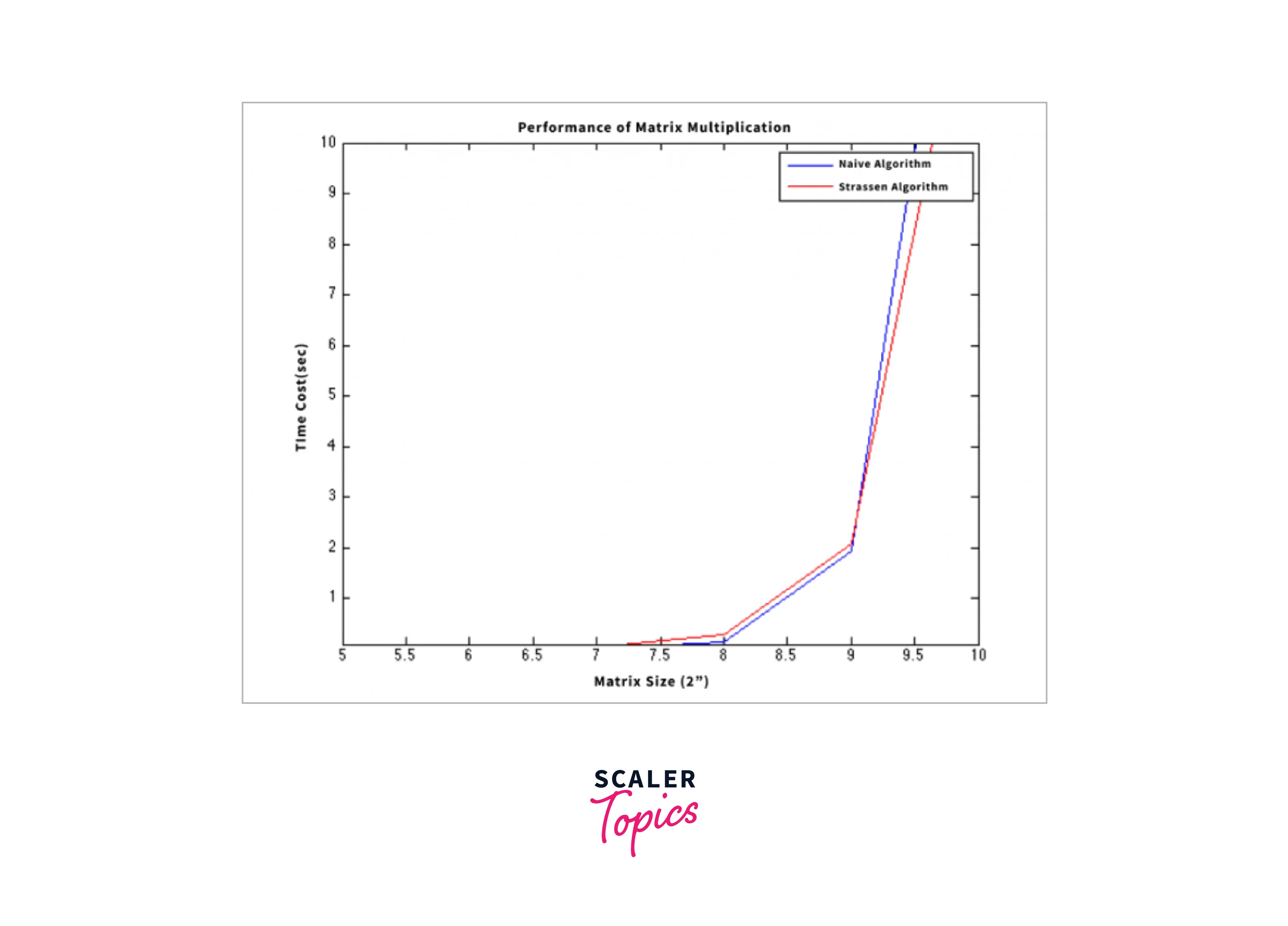
• Therefore we can observe that Strassen’s Matrix Multiplication algorithm is considered to be efficient for matrix multiplication.

Space Complexity: O(log N), where the given matrices are square matrices of size N*N each. The submatrices in recursion take extra space.

Easy Method to Remember Strassen’s Matrix Equations

Strassen's Matrix Multiplication has 7 recursive calls and computing the values in the resultant matrix. Below are a few ways used for remembering how to compute the values required to fill the resultant matrix.

• Consider the below image:
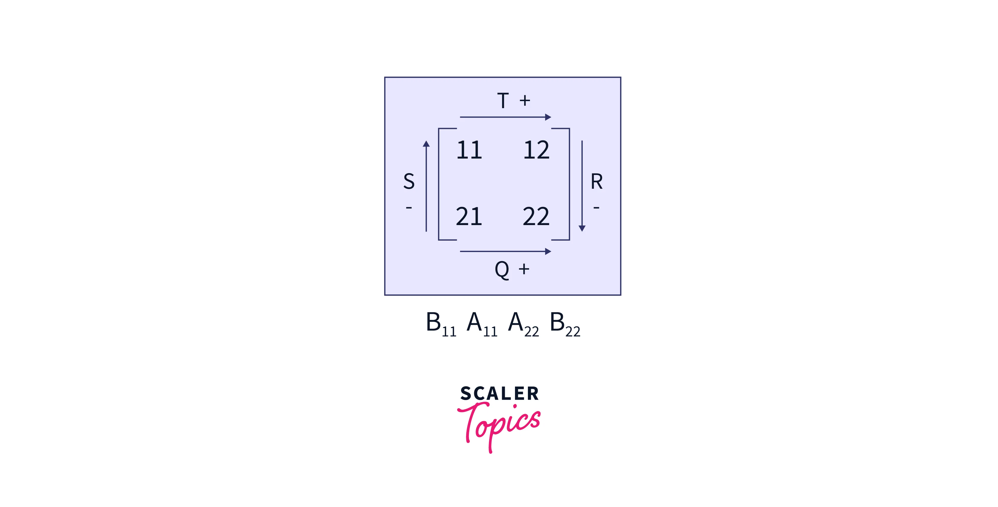
• For calculating the values of P, we just need to multiply the product of the sum of the diagonal elements.
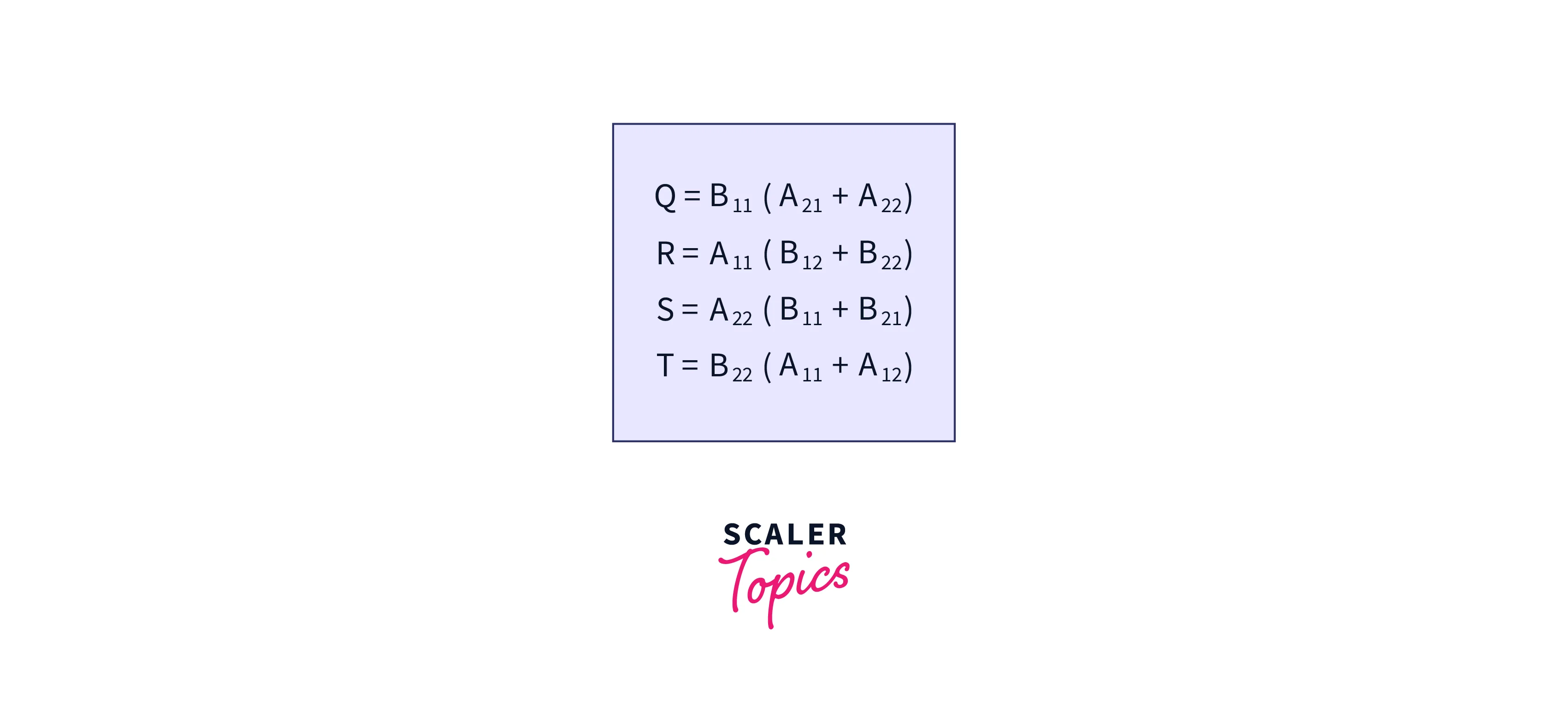
• For writing the values of Q, R, S and T follow the below steps:
• Place the initial values as shown in the figure:
• Now for computing the values of Q, R, S, and T we just need to check whether the initial value's coefficient we have taken as in the above image is either A or B. If B is taken, then in the brackets we need to have A as the coefficient, whereas if the initial coefficient taken is A as shown in the figure, then the values in the bracket should be of coefficient B.
• Now to fill the values taking the reference from image 6, we can say that for T and Q, we need to add the values shown by the arrow direction.
• Whereas for computing the values of S and R, we need to subtract the values indicated by the arrow in the image6.
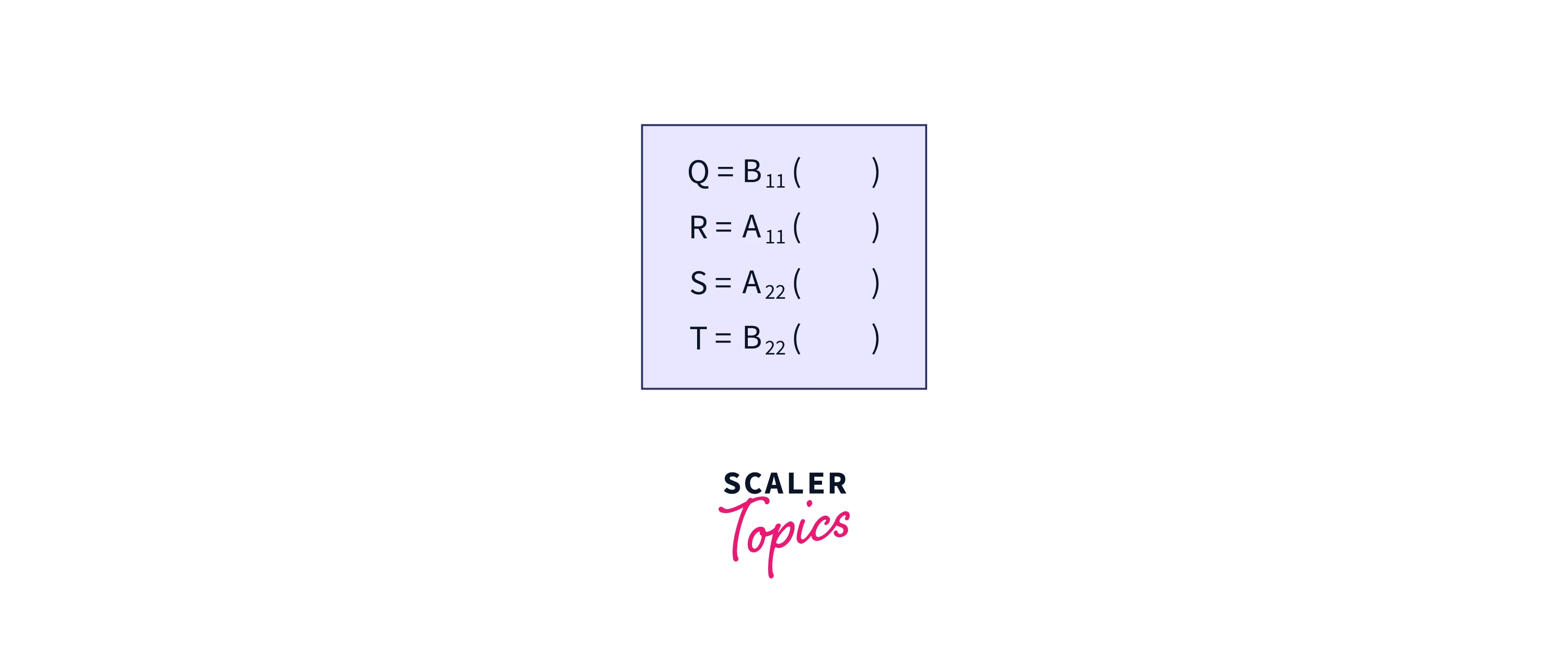
• The equation of Q, R, S and T can be shown in the below image:
• Last step includes calculating the values of U, here we use the values of S and T. We need to toggle the coefficients i.e, A becomes B and B becomes A. So U obtained is as follows: $U=~(A_{21})~*~(A_{11})~*~(B_{11}~+~B_{12})$
• Similarly, value of V is obtained by using the values of Q and R. Here we just need to toggle A and B present in the brackets. Therefore the value of V is: $V~=~(B_{21}~+~B_{22})~*~(A_{12}~-~A_{22})$.
• After computing the values of P, Q, R, S, T, U, V. We need to calculate the values of $C_{11},~ C_{12},~ C_{21},~ C_{22}$ which are the values of resultant matrix.
• We need to calculate them in the following way:
  • $C_{11} =~ P~ +~ S~ -~T~ +~ V$
  • $C_{12} ~= ~R ~+ ~T$
  • $C_{21} ~= ~Q ~+ ~S$
  • $C_{22} = P + R - Q + U$

Invest in your programming future with our in-depth Dynamic Programming Certification Course. Enroll now and supercharge your coding skills!