Time Series Analysis in R

Introduction

Time Series Analysis in R is a vital statistical technique for comprehending and predicting temporal data patterns. Time series data consists of observations collected at specific time intervals, such as daily stock prices, monthly sales figures, or hourly temperature readings. R, a widely-used programming language for data analysis and visualisation, offers an array of packages and functions tailored for effective time series exploration.

The primary steps in Time Series Analysis R involve:

• Data Import and Preprocessing: Loading time-stamped data into R using packages like "xts" or "zoo," which provide specialised data structures for handling time series. Cleaning and formatting the data for analysis is crucial.
• Exploratory Analysis: Visualising the time series data through plots, graphs, and summary statistics to identify trends, seasonality, and potential outliers. The "ggplot2" package can be useful for creating informative visualisations.
• Decomposition: Decomposing the time series into its components—trend, seasonality, and residual—using techniques like additive or multiplicative decomposition. This step aids in understanding the underlying patterns.
• Smoothing and Filtering: Applying moving averages or exponential smoothing techniques to remove noise and emphasise underlying trends or seasonal fluctuations.
• Modelling: Employing statistical models like ARIMA (AutoRegressive Integrated Moving Average) or SARIMA (Seasonal ARIMA) to capture and predict patterns in the time series data.
• Forecasting: Utilising the "forecast" package to generate forecasts based on the chosen model. This helps in predicting future values and their associated uncertainties.
• Model Evaluation: Assessing the model's accuracy using metrics like Mean Absolute Error (MAE), Root Mean Squared Error (RMSE), or Mean Absolute Percentage Error (MAPE). Cross-validation techniques ensure the model's robustness.
• Interpretation and Communication: Deriving insights from the analysis and communicating findings effectively through reports, visualisations, and dashboards.

What is Time Series Analysis?

Time Series Analysis is a statistical technique used to analyse and interpret data points that are collected at regular intervals over time. These data points could be measurements, observations, or readings taken sequentially, such as daily stock prices, monthly sales figures, hourly temperature readings, or annual GDP growth rates.

The goal of Time Series Analysis is to uncover patterns, trends, and underlying structures within the data. It involves exploring how these patterns change over time, identifying any seasonality or cyclic behaviour, and understanding how past observations can help predict future values. This analysis is valuable for making informed decisions, forecasting future trends, and gaining insights into the dynamics of various phenomena, ranging from financial markets to environmental changes.

By studying the temporal relationships and characteristics of time series data, analysts can derive valuable insights that inform strategies, policies, and business decisions. Techniques such as decomposition, smoothing, and modelling are commonly employed to extract meaningful information from time series data, aiding in understanding the complexities of real-world processes evolving over time.

Understanding Time Series Components

Time series data consists of observations collected over time. To understand the underlying structure and patterns within such data, it's crucial to break down the time series into its key components:

• Trend: The trend component represents the long-term movement or direction in the data. It indicates whether the data is generally increasing, decreasing, or remaining relatively stable over time. Trends can be linear, nonlinear, or even cyclic. Identifying the trend helps in understanding the overall behaviour of the data.
• Seasonality: Seasonality refers to patterns that repeat at regular intervals, often corresponding to seasons, months, weeks, or even days of the week. Seasonal patterns can arise due to external factors, such as holidays, weather, or economic cycles. Recognizing seasonality is crucial for predicting and addressing cyclic variations in the data.
• Cyclic Patterns: Unlike seasonality, cyclic patterns do not have fixed periodicity and can extend beyond a single year. These patterns are often influenced by economic or business cycles and may not repeat at consistent intervals. Cycles can be longer and less predictable than seasonal patterns.
• Irregular or Residual Component: This component captures the random fluctuations and noise present in the data that cannot be attributed to the trend, seasonality, or cyclic behaviour. These fluctuations can arise due to unforeseen events, measurement errors, or other sources of variability.

How to create a Time Series in R ?

Creating a time series in R involves using appropriate functions and data structures to organise and represent the temporal data. Here's an example of how to create a simple time series in R using the built-in dataset "AirPassengers," which contains monthly airline passenger numbers from 1949 to 1960:

Explanation of the steps:

• The library(tseries) line loads the "tseries" package, which provides functions for time series analysis.
• The data("AirPassengers") line loads the "AirPassengers" dataset included in the package. This dataset contains the monthly passenger counts.
• The ts() function is used to convert the loaded dataset into a time series object. The start parameter specifies the starting time period (January 1949 in this case), and the frequency parameter indicates that the data is collected monthly (frequency = 12).
• The print(passengers_ts) line prints the created time series object, which will display the monthly passenger counts over the specified time period.

Output:

Different Time intervals

Time series data can be collected at various time intervals, ranging from very short intervals, such as milliseconds, to longer intervals, like years. R provides tools to handle different time intervals in time series analysis using appropriate packages and functions. Here are some common time intervals and how to work with them in R:

Daily Time Series:

In this example, replace data with your dataset, start_date with the starting date, and set the frequency to 365 for daily data.

Monthly Time Series:

Set the frequency to 12 for monthly data.

Quarterly Time Series:

Use a frequency of 4 for quarterly data.

Annual Time Series:

Set the frequency to 1 for annual data.

Irregular Time Series (Time Stamps):

Output:

For irregular data with timestamps, use the ts() function with the start parameter set to the first timestamp.

Multiple Time series in R.

Working with multiple time series in R involves managing and analysing multiple datasets that are collected over time. You can use various packages like "xts," "zoo," and "tsibble" to handle and analyse multiple time series efficiently. Here's an example of how to work with multiple time series using the "xts" package:

Load Required Packages:

library(xts)

Create Multiple Time Series:

Access and Manipulate Time Series:

Plot Multiple Time Series:

In this example, we created two time series (TimeSeries1 and TimeSeries2) using the "xts" package, performed calculations on them, subsetted them based on date ranges, and plotted them together. You can further extend your analysis by incorporating various time series analysis techniques, forecasting models, and visualisations to gain insights from multiple time series data.

What is a Stationarity in Time Series?

Stationarity is a fundamental concept in time series analysis. A time series is considered stationary when its statistical properties do not change over time. In other words, the mean, variance, and autocorrelation structure remain constant across different time periods. Stationarity is a crucial assumption in many time series models and analyses, as non-stationary data can lead to misleading results and inaccurate predictions.

There are two main components of stationarity:

1. Strict Stationarity: A time series is strictly stationary if the joint distribution of any set of time points is the same as the joint distribution of the same set of time points shifted by a constant time interval. In other words, the statistical properties of the data remain unchanged regardless of the time window being considered.
2. Weak Stationarity (also known as Wide-Sense Stationarity): A time series is weakly stationary if its mean, variance, and autocorrelation function (ACF) are constant over time. This is a more practical and commonly used form of stationarity. It allows for some variations in the data, but these variations are not systematic and do not introduce trends or patterns.

Stationary Data Example:

Stationary data remains relatively constant over time, without any discernible trend or seasonality.

Output:

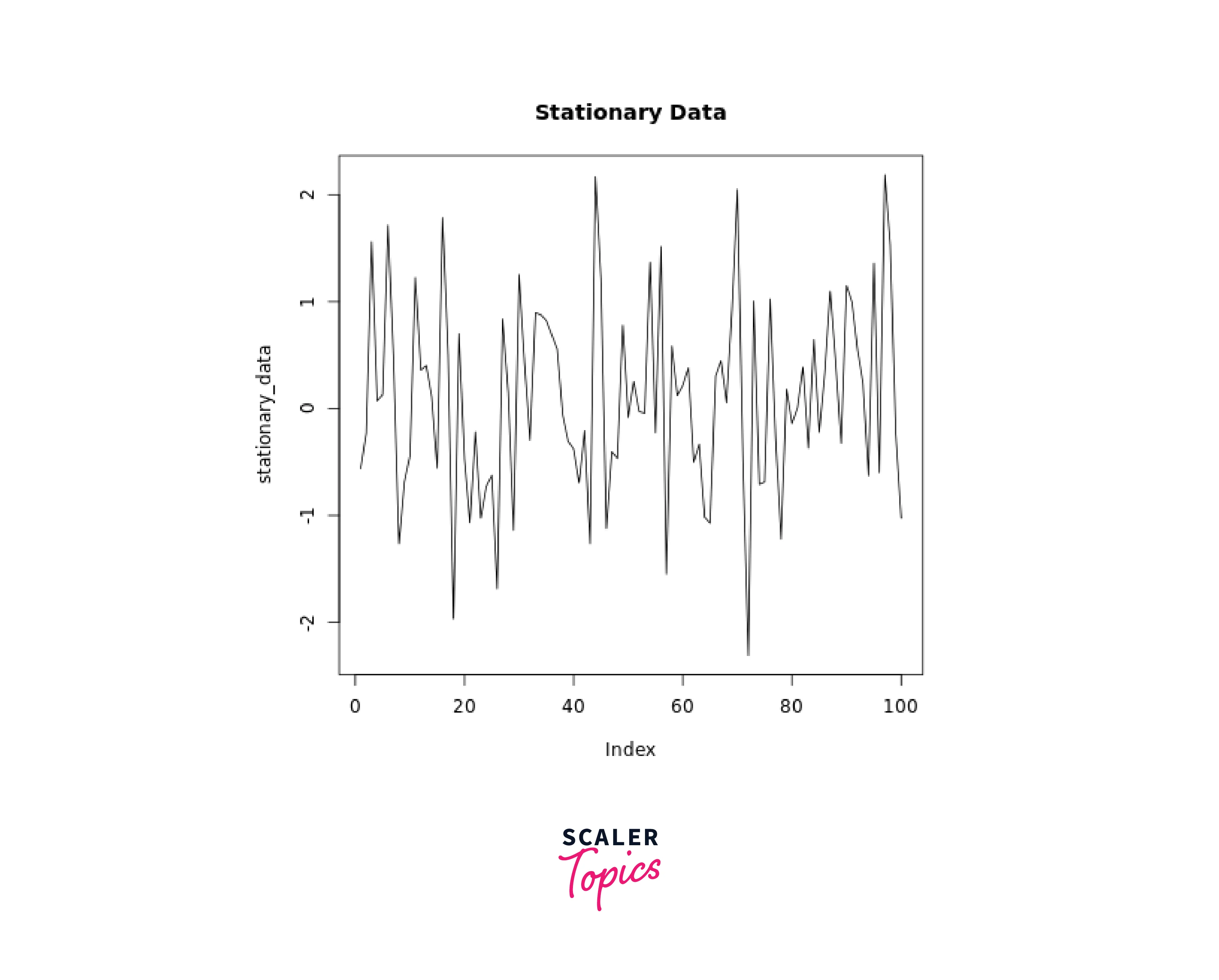
In this example, the generated stationary data follows a normal distribution and shows no clear upward or downward trend.

Non-Stationary Data Example:

Non-stationary data exhibits trends, seasonality, or other patterns that change over time.

Output:

In this example, the generated non-stationary data includes a clear linear increasing trend along with random noise.

Illustration Summary:

The key difference between stationary and non-stationary data is the presence of trends, seasonality, or other patterns that change over time in non-stationary data. Stationary data, on the other hand, remains relatively consistent over time.

By visually comparing the plots of the stationary and non-stationary data, you can observe how the behavior of the two time series differs. In real-world scenarios, identifying whether your data is stationary or non-stationary is essential for selecting appropriate time series analysis techniques and models.

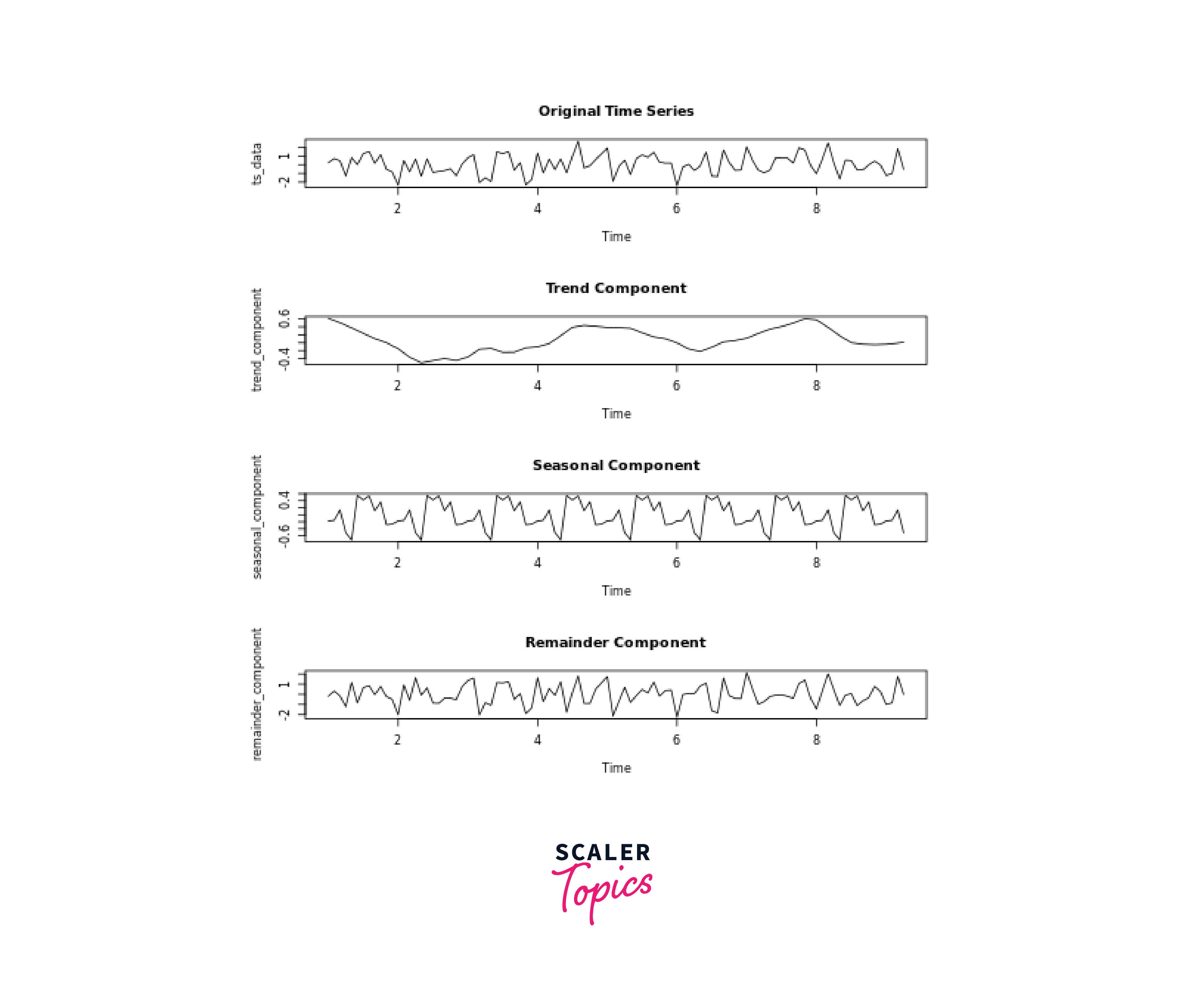
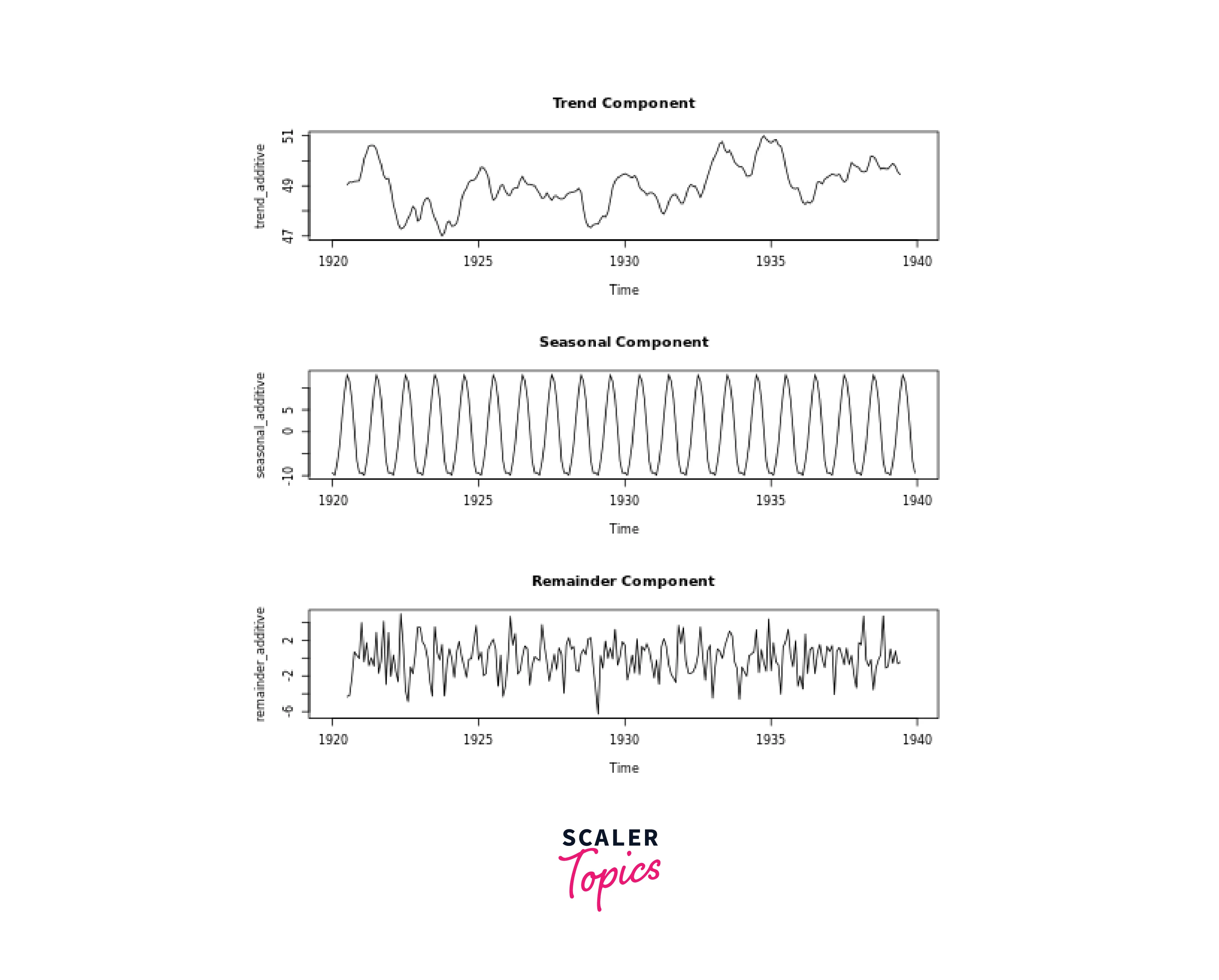
Extracting the trend, seasonality/Decomposition in R

In R, you can extract the trend and seasonality components from a time series using various functions and packages. Here's how you can perform decomposition to extract trend and seasonality using the "decompose" function, which is part of the base R package:

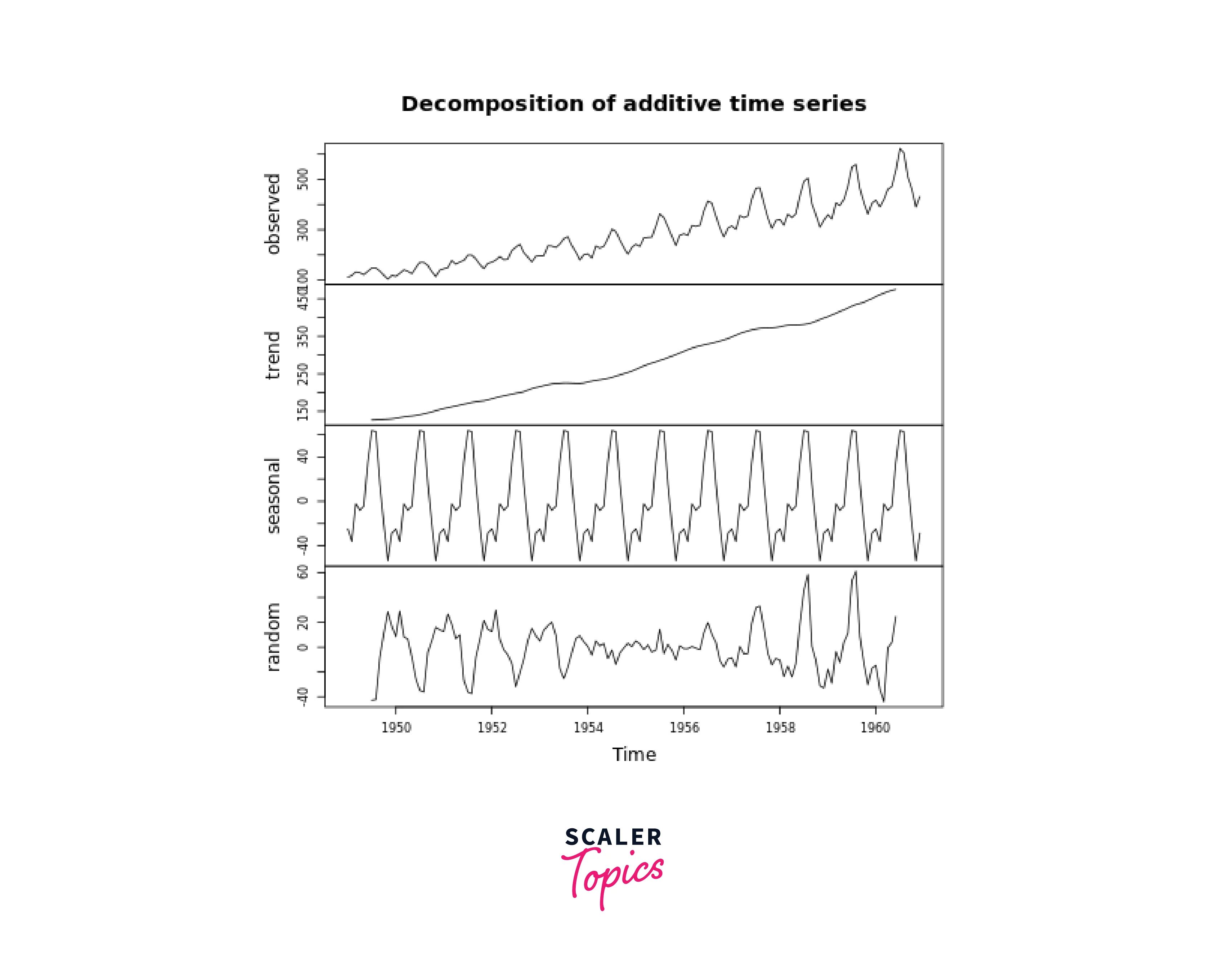Here's an alternative method using the "stl" function from the "stats" package, which provides more advanced decomposition with better handling of seasonal components:

In both methods, ts_data is your time series data, and the trend_component, seasonal_component, and remainder_component will store the extracted components. The "decompose" function provides basic decomposition, while the "stl" function offers more sophisticated decomposition with improved handling of irregular seasonality.

Output:

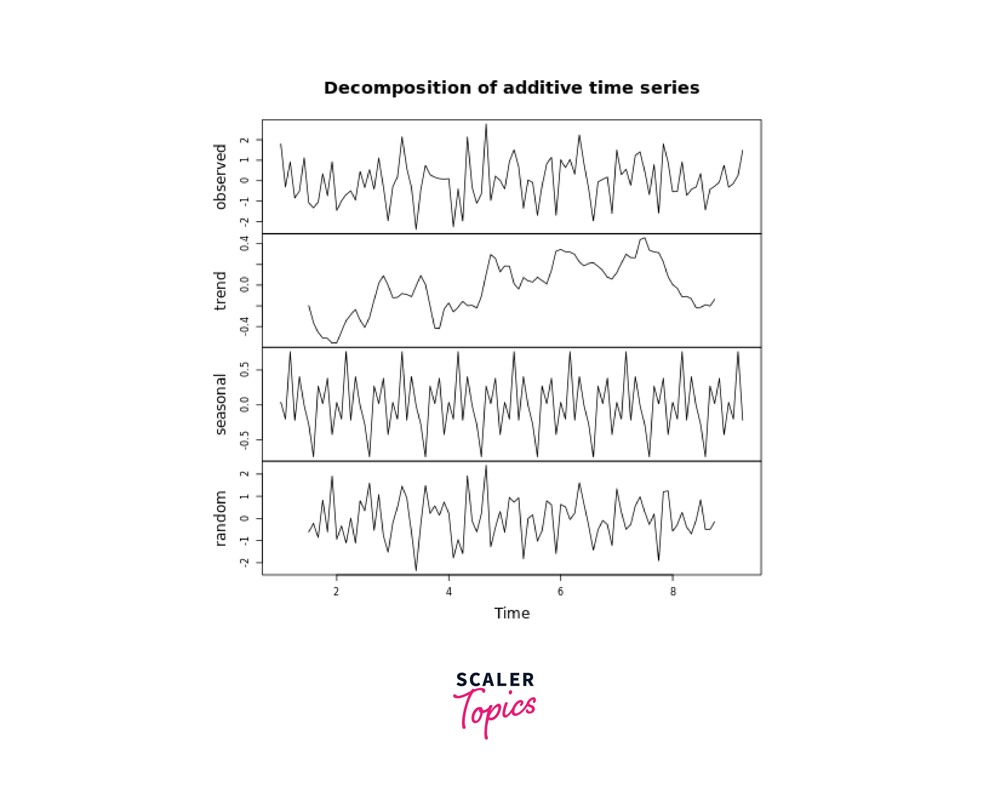
Additive and Multiplicative Decomposition

Additive and multiplicative decomposition are two common methods used to decompose time series data into its trend, seasonality, and residual components. The choice between additive and multiplicative decomposition depends on whether the magnitude of seasonality varies with the level of the data (multiplicative) or remains constant (additive).

Here's how you can perform additive and multiplicative decomposition in R using the "decompose" function:

Additive Decomposition: Additive decomposition assumes that the magnitude of seasonality remains constant across different levels of the data.

Output: Multiplicative Decomposition: Multiplicative decomposition assumes that the magnitude of seasonality changes with the level of the data.

In both cases, replace ts_data with your actual time series data. The decompose function from the base R package performs the decomposition based on the specified type ("additive" or "multiplicative"). You can access the extracted components using the respective names (trend, seasonal, random), which are stored in the returned object.

Output:

Time Series Decomposition Using decompose()

Certainly! The decompose() function in R is a convenient way to perform time series decomposition. It decomposes a time series into its components: trend, seasonality, and remainder. Here's how you can use the decompose() function:

In this example, the decompose() function is applied to the "nottem" dataset, which contains monthly average temperatures. The decomposition type is set to "additive." You can replace ts_data with your own time series data.

The trend, seasonal, and random components are accessed using the corresponding names in the returned object. The resulting plots display the trend, seasonality, and remainder components separately.

Output:

Time Series Modeling and Forecasting

Time series modelling and forecasting involve selecting appropriate models to capture underlying patterns and using those models to predict future values. Here's an overview of key concepts and methods:

1. Selecting and Fitting Time Series Models:

• Data Understanding: Analyze trends, seasonality, and noise in your data.
• Model Selection: Choose models based on data patterns and characteristics. Consider ARIMA, Exponential Smoothing, and SARIMA.
• Model Fitting: Estimate model parameters using historical data.

2. Autoregressive Integrated Moving Average (ARIMA) Models:

• Strengths: Good for capturing linear trends and autocorrelation patterns.
• Trade-offs: May not handle nonlinear trends or complex seasonality well.

3. Exponential Smoothing Models:

• Strengths: Weights recent observations, suitable for data with evolving patterns.
• Trade-offs: May not capture complex seasonality or long-term trends.

4. Seasonal ARIMA (SARIMA) Models:

• Strengths: Handles seasonality and autocorrelation effectively.
• Trade-offs: Requires a good understanding of the data and can be complex to configure.

5. Handling Seasonality and Trend in Forecasting:

• Detrending: Removes trend, making data stationary.
• Differencing: Removes seasonality and stabilizes variance.
• Decomposition: Separates trend, seasonality, and residuals for analysis.

6. Forecasting Steps:

• Model Selection: Choose the appropriate model based on data characteristics.
• Model Fitting: Estimate model parameters using historical data.
• Forecasting: Generate forecasts for future time periods.
• Evaluation: Assess forecast accuracy using metrics like MAE, RMSE, or MAPE.
• Tuning: Adjust model parameters to optimize accuracy.
• Visualization: Plot forecasts with historical data for insights.
• Uncertainty Analysis: Determine confidence intervals for forecast ranges.

Trade-offs Between Models:

• Complexity: More complex models like SARIMA may be harder to interpret and require more computational resources.
• Interpretability: Simpler models like Exponential Smoothing can be more easily understood.
• Data Requirements: ARIMA and SARIMA may need large amounts of historical data to estimate parameters accurately.
• Seasonality Handling: SARIMA is specifically designed for seasonal data, while Exponential Smoothing models can adapt to evolving patterns.
• Model Assumptions: Each model has specific assumptions; failing to meet them can lead to inaccurate forecasts.